ResNet (34, 50, 101): Residual CNNs for Image Classification Tasks

ResNet is a short name for a residual network, but what’s residual learning?

Deep convolutional neural networks have achieved the human level image classification result. Deep networks extract low, middle and high-level features and classifiers in an end-to-end multi-layer fashion, and the number of stacked layers can enrich the “levels” of features.  The stacked layer is of crucial importance, look at the ImageNet result.

When the deeper network starts to converge, a degradation problem has been exposed: with the network depth increasing, accuracy gets saturated (which might be unsurprising) and then degrades rapidly. Such degradation is not caused by overfitting or by adding more layers to a deep network leads to higher training error. The deterioration of training accuracy shows that not all systems are easy to optimize.

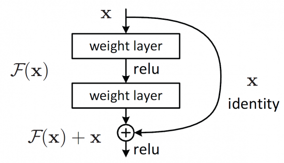
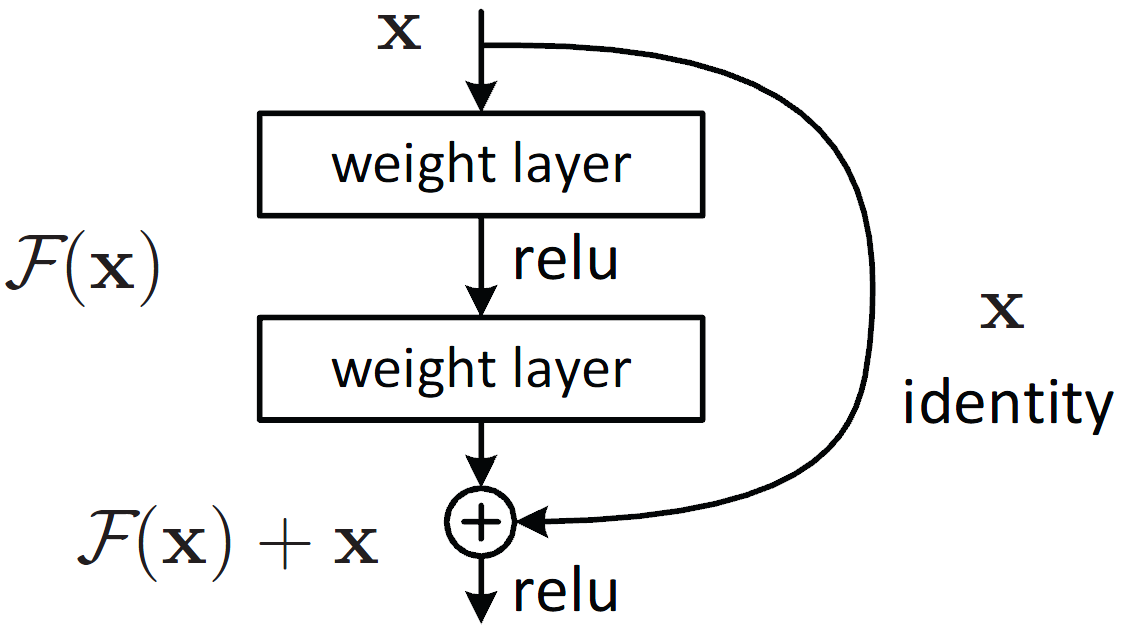
To overcome this problem, Microsoft introduced a deep residual learning framework. Instead of hoping every few stacked layers directly fit a desired underlying mapping, they explicitly let these layers fit a residual mapping. The formulation of F(x)+x can be realized by feedforward neural networks with shortcut connections. Shortcut connections are those skipping one or more layers shown in Figure 1. The shortcut connections perform identity mapping, and their outputs are added to the outputs of the stacked layers. By using the residual network, there are many problems which can be solved such as:

• ResNets are easy to optimize, but the “plain” networks (that simply stack layers) shows higher training error when the depth increases.
• ResNets can easily gain accuracy from greatly increased depth, producing results which are better than previous networks.

Datasets

ImageNet is a dataset of millions of labeled high-resolution images belonging roughly to 22k categories. The images were collected from the internet and labeled by humans using a crowd-sourcing tool. Starting in 2010, as part of the Pascal Visual Object Challenge, an annual competition called the ImageNet Large-Scale Visual Recognition Challenge (ILSVRC2013) has been held. ILSVRC uses a subset of ImageNet with roughly 1000 images in each of 1000 categories. There are approximately 1.2 million training images, 50k validation, and 150k testing images.

The PASCAL VOC provides standardized image data sets for object class recognition. It also provides a standard set of tools for accessing the data sets and annotations, enables evaluation and comparison of different methods and ran challenges evaluating performance on object class recognition.

Architecture

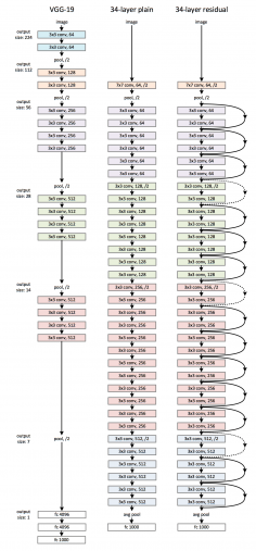
Plain Network: The plain baselines (Fig. 2, middle) are mainly inspired by the philosophy of VGG nets (Fig. 2, left). The convolutional layers mostly have 3×3 filters and follow two simple rules:

1. For the same output feature map, the layers have the same number of filters;
2. If the size of the features map is halved, the number of filters is doubled to preserve the time complexity of each layer.

It is worth noticing that the ResNet model has fewer filters and lower complexity than VGG nets.

Residual Network: Based on the above plain network, a shortcut connection is inserted (Fig. 2, right) which turn the network into its counterpart residual version. The identity shortcuts F(x{W}+x) can be directly used when the input and output are of the same dimensions (solid line shortcuts in Fig. 2). When the dimensions increase (dotted line shortcuts in Fig. 2), it considers two options:

1. The shortcut performs identity mapping, with extra zero entries padded for increasing dimensions. This option introduces no additional parameter.
2. The projection shortcut in F(x{W}+x) is used to match dimensions (done by 1×1convolutions).

For either of the options, if the shortcuts go across feature maps of two size, it performed with a stride of 2.

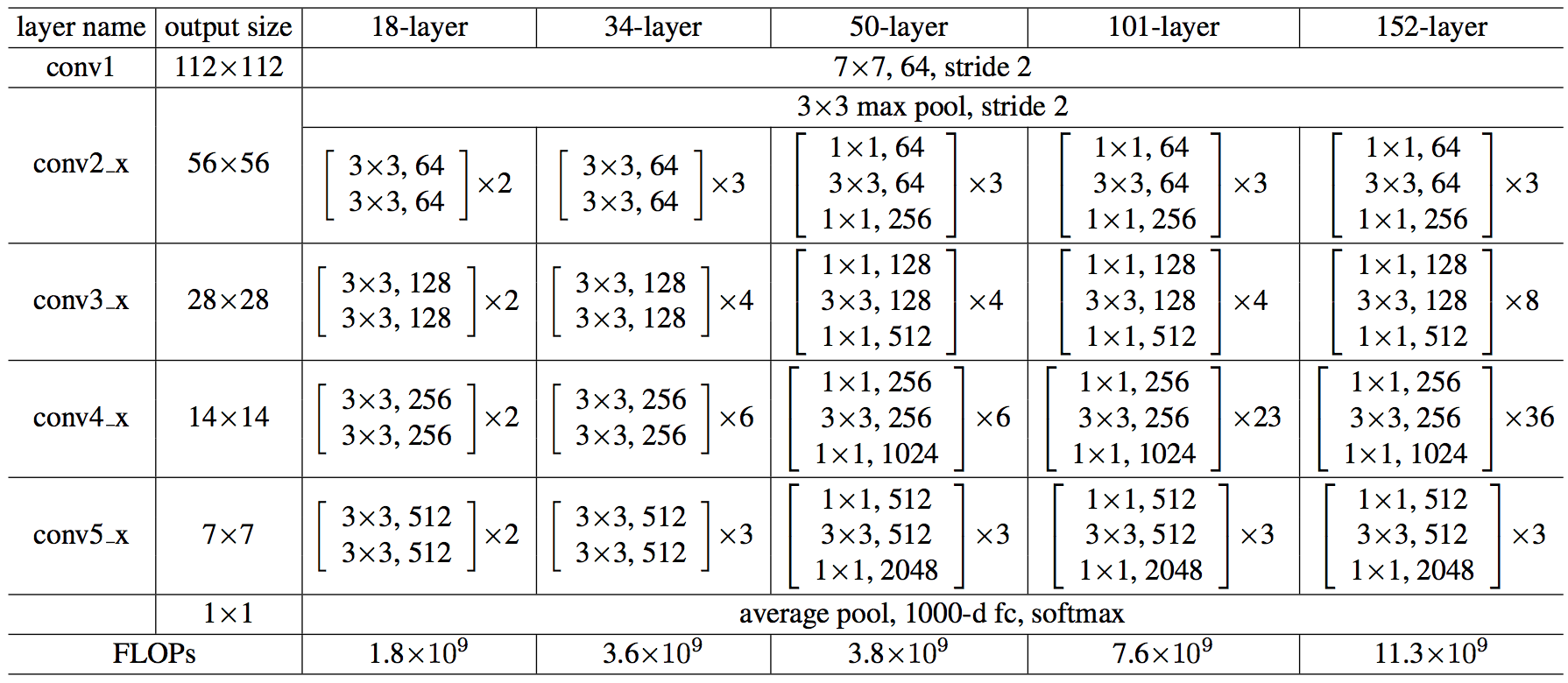
Each ResNet block is either two layers deep (used in small networks like ResNet 18, 34) or 3 layers deep (ResNet 50, 101, 152).

50-layer ResNet: Each 2-layer block is replaced in the 34-layer net with this 3-layer bottleneck block, resulting in a 50-layer ResNet (see above table). They use option 2 for increasing dimensions. This model has 3.8 billion FLOPs.

101-layer and 152-layer ResNets: they construct 101-layer and 152-layer ResNets by using more 3-layer blocks (above table). Even after the depth is increased, the 152-layer ResNet (11.3 billion FLOPs) has lower complexity than VGG-16/19 nets (15.3/19.6 billion FLOPs)

Implementation

The image is resized with its shorter side randomly sampled in [256,480] for scale augmentation. A 224×224 crop is randomly sampled from an image or its horizontal flip, with the per-pixel mean subtracted.  The learning rate starts from 0.1 and is divided by 10 when the error plateaus and the models are trained for up to 60×10000 iterations. They use a weight decay of 0.0001 and a momentum of 0.9.
[Pytorch][Tensorflow][Keras]

Result

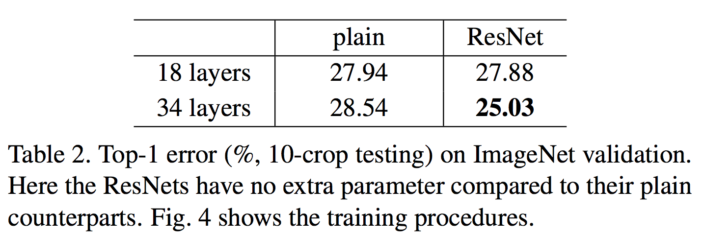
The 18 layer network is just the subspace in 34 layer network, and it still performs better. ResNet outperforms with a significant margin in case the network is deeper.

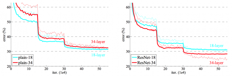
ResNet network converges faster compared to the plain counterpart of it. Figure 4 shows that the deeper ResNet achieve better training result as compared to the shallow network.

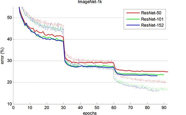
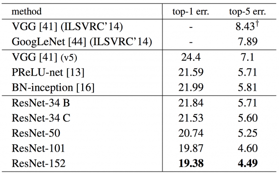
ResNet-152 achieves a top-5 validation error of 4.49%. A combination of 6 models with different depths achieves a top-5 validation error of 3.57%. Winning the 1st place in ILSVRC-2015