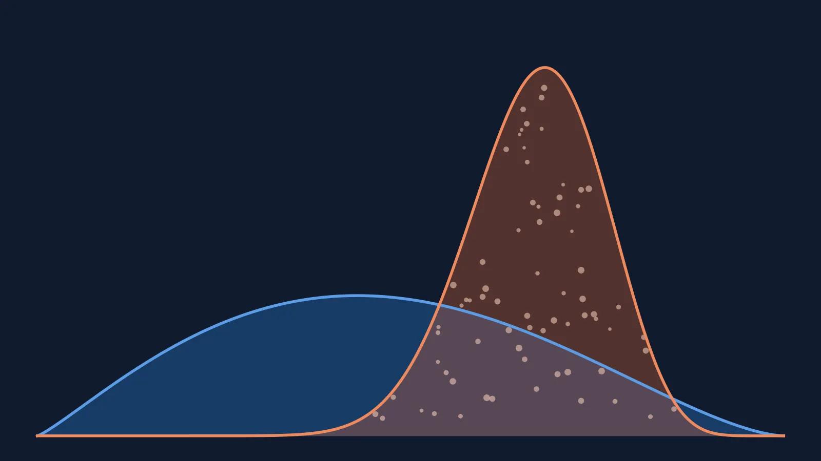
Bayes’ theorem tells you how to update a probability when new evidence arrives: the probability of a hypothesis given the evidence equals the probability of the evidence given the hypothesis, times the prior probability of the hypothesis, divided by the overall probability of the evidence. In symbols, P(H | E) = P(E | H) · P(H) / P(E). It is the reason a positive result on a 95%-accurate test can still mean only a 16% chance of being sick, and it is the core of spam filters, Naive Bayes classifiers and Bayesian inference in machine learning.
This guide explains the formula in plain English, derives it in three lines, walks through two worked examples with real numbers, and shows how to compute everything in Python.
Key takeaways
- Formula: posterior = likelihood × prior / evidence.
- Prior P(H) is what you believed before; posterior P(H | E) is what you believe after seeing the evidence.
- The base rate matters most: when a condition is rare, even an accurate test produces more false alarms than true hits.
- Bayes’ theorem, Bayes’ rule, Bayes’ law and Bayes’ formula are four names for the same equation.
- In machine learning it powers Naive Bayes classifiers, Bayesian inference and Bayesian hyperparameter optimization.
What Is Bayes’ Theorem?
Bayes’ theorem is a rule from probability theory for reversing a conditional probability. You often know how likely the evidence is if a hypothesis is true — how often a test is positive when someone is sick, how often the word “free” appears in spam — but what you actually want is the opposite: how likely the hypothesis is now that you have seen the evidence. Bayes’ theorem converts one into the other.
The idea is named after Thomas Bayes, an English minister and mathematician. His essay on the problem was found after his death in 1761 and presented to the Royal Society by his friend Richard Price in 1763. Pierre-Simon Laplace arrived at the same result independently in 1774 and developed it into the general method that statisticians use today.
You will see the same equation called Bayes’ rule, Bayes’ law or Bayes’ formula. There is no difference between them.
The Bayes’ Theorem Formula
For a hypothesis H and evidence E:
P(H | E) = P(E | H) · P(H) / P(E)
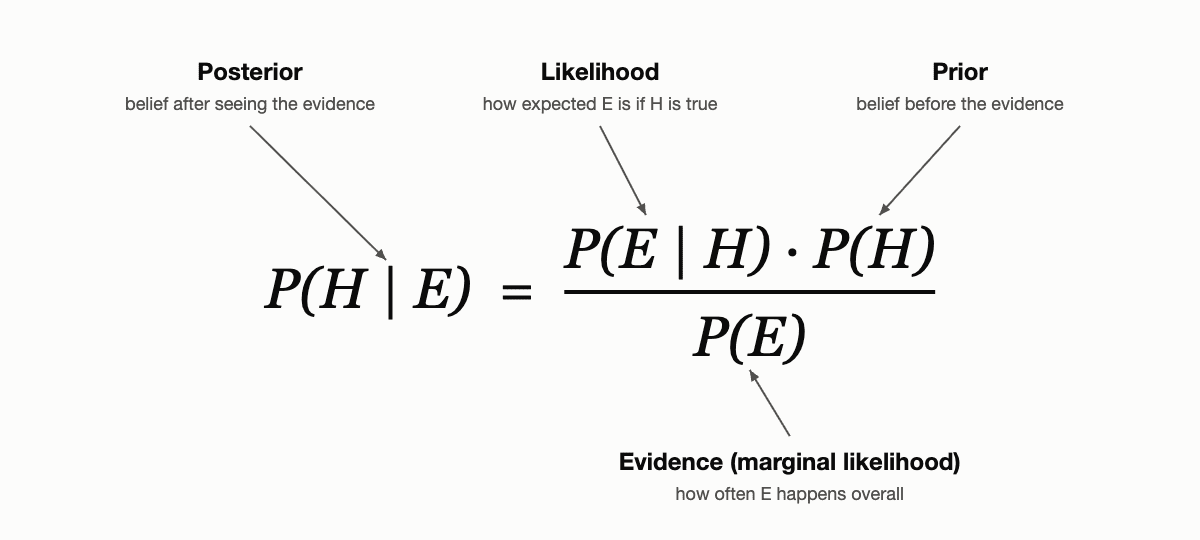
| Term | Name | What it means | Medical-test example |
|---|---|---|---|
| P(H) | Prior | Probability of the hypothesis before you see the evidence | 1% of people have the disease |
| P(E | H) | Likelihood | Probability of the evidence if the hypothesis is true | 95% of sick people test positive |
| P(E) | Evidence (marginal likelihood) | Overall probability of the evidence, whether or not H is true | 5.9% of all tests are positive |
| P(H | E) | Posterior | Probability of the hypothesis after you see the evidence | 16.1% of positives are actually sick |
The vertical bar reads as “given”. P(H | E) is “the probability of H given E”. The single most useful habit with Bayes’ theorem is to notice that P(H | E) and P(E | H) are different numbers — often wildly different.
The denominator is usually the hardest part to find directly. It is computed with the law of total probability: the evidence can occur either when H is true or when it is false, so
P(E) = P(E | H) · P(H) + P(E | not H) · P(not H)
Substituting this into the formula gives the version you will use most often in practice:
P(H | E) = P(E | H) · P(H) / [P(E | H) · P(H) + P(E | not H) · (1 − P(H))]
Where the Formula Comes From
Bayes’ theorem is not an extra assumption. It follows directly from the definition of conditional probability: the probability that both H and E happen equals the probability of one event times the probability of the other given the first.
- P(H and E) = P(H | E) · P(E)
- P(H and E) = P(E | H) · P(H)
- Both right-hand sides equal the same thing, so P(H | E) · P(E) = P(E | H) · P(H). Divide by P(E) and you get Bayes’ theorem.
That is the whole proof. Everything else — Naive Bayes, Bayesian networks, Bayesian inference — is this one identity applied carefully.
Example 1: A Positive Medical Test
This is the classic example, and the one that surprises people most. Suppose:
- 1% of the population has a disease (the prior, or base rate);
- the test detects 95% of real cases (sensitivity, P(positive | sick) = 0.95);
- it correctly clears 95% of healthy people (specificity), so 5% of healthy people get a false positive.
You test positive. What is the chance you actually have the disease? Most people guess about 95%. Bayes’ theorem says:
P(sick | positive) = 0.95 × 0.01 / (0.95 × 0.01 + 0.05 × 0.99) = 0.0095 / 0.059 ≈ 16.1%
The easiest way to see why is to count people instead of multiplying probabilities. Imagine testing 10,000 people:
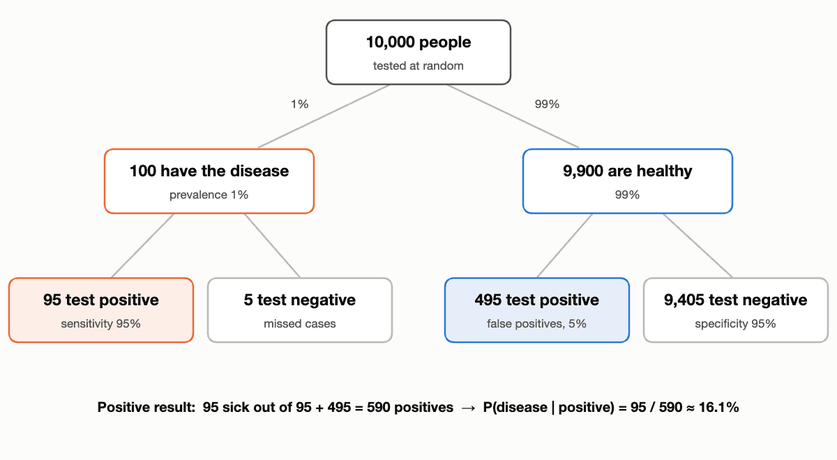
Only 100 people are sick, and 95 of them test positive. But 9,900 people are healthy, and 5% of them — 495 people — also test positive. Out of 590 positive results, only 95 belong to sick people. The test is good; the disease is simply rare, so false alarms from the large healthy group swamp the true hits. Ignoring this effect is called the base rate fallacy.
The prior has an enormous effect on the answer. The chart below shows the posterior for the same positive result across different prevalence levels:
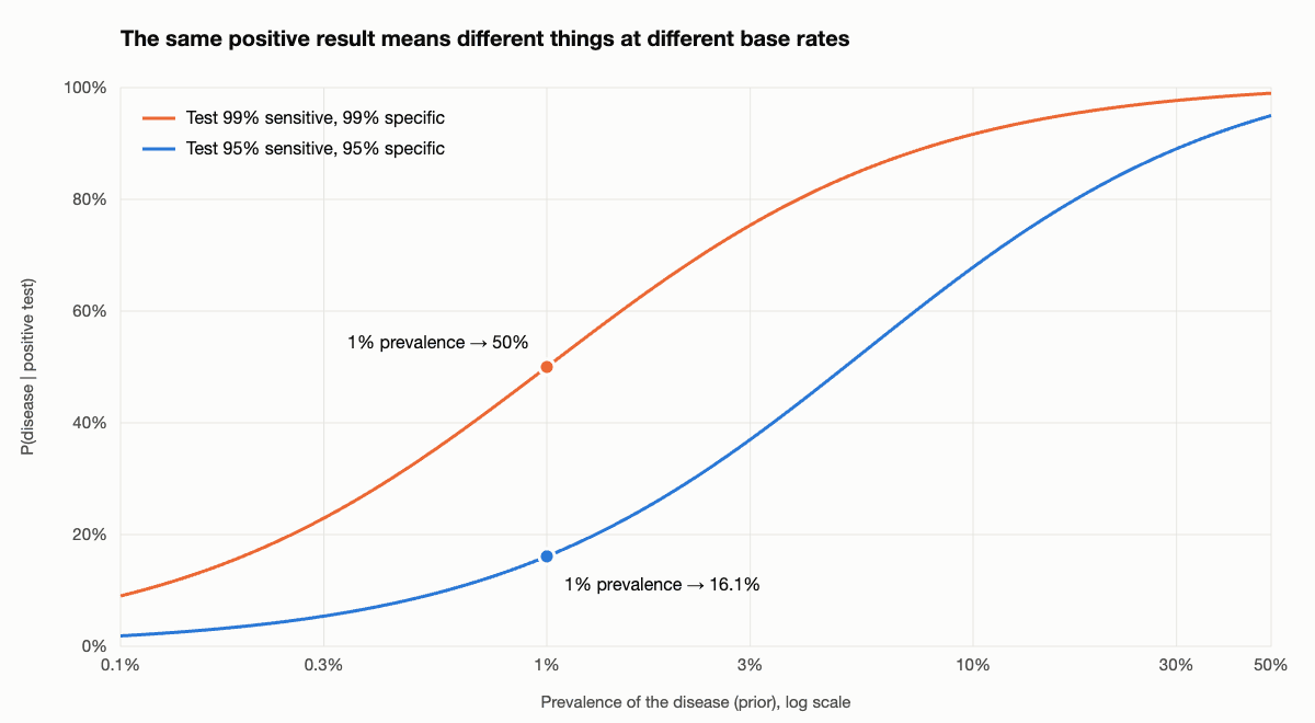
This is why doctors confirm screening results with a second, independent test, and why a test is far more informative when it is ordered because of symptoms (a higher prior) than when it is run on everyone.
Example 2: Is This Email Spam?
Spam filtering was one of the first large-scale applications of Bayes’ theorem in software. Suppose, from your mailbox history:
- 40% of incoming email is spam: P(spam) = 0.40;
- the word “free” appears in 25% of spam: P(free | spam) = 0.25;
- it appears in only 2% of legitimate email: P(free | not spam) = 0.02.
A new message contains “free”. The probability that it is spam is:
P(spam | free) = 0.25 × 0.40 / (0.25 × 0.40 + 0.02 × 0.60) = 0.100 / 0.112 ≈ 89.3%
One word moved the estimate from 40% to 89%. A real filter combines evidence from hundreds of words at once, which is exactly what the Naive Bayes classifier further down does.
Bayesian Updating: Today’s Posterior Is Tomorrow’s Prior
The posterior from one calculation becomes the prior for the next. Go back to the medical test and take a second, independent test that also comes back positive. The new prior is no longer 1% — it is the 16.1% you just computed:
P(sick | two positives) = 0.95 × 0.161 / (0.95 × 0.161 + 0.05 × 0.839) ≈ 78.5%
Two positive results take you from 1% to 78.5%. A negative first test, by contrast, drops the probability from 1% to about 0.05%. This step-by-step revision of beliefs as data arrives is called Bayesian updating, and it is how Bayesian models in statistics and machine learning learn from data.
The updates are only this simple when the tests are independent given the true state. Two runs of the same test on the same sample usually share their errors, so in that case the second result adds much less information than the formula suggests.
The Odds Form: A Shortcut for Mental Math
Bayes’ theorem has an equivalent form that is easier to compute in your head:
posterior odds = prior odds × likelihood ratio
The likelihood ratio is P(E | H) / P(E | not H). For the medical test it is 0.95 / 0.05 = 19, so a positive result multiplies the odds of disease by 19. The prior odds are 1 : 99. Multiplying gives posterior odds of 19 : 99, which is 19 / (19 + 99) ≈ 16.1% — the same answer, with no denominator to compute. Each additional independent test simply multiplies the odds by its own likelihood ratio.
Bayes’ Theorem in Python
A Bayes’ theorem calculator is a few lines of code. This function takes the prior, the probability of the evidence when the hypothesis is true, and the probability of the evidence when it is false:
def posterior(prior, p_e_given_h, p_e_given_not_h):
    """Bayes' theorem: P(H | E) from P(H), P(E | H) and P(E | not H)."""
    evidence = p_e_given_h * prior + p_e_given_not_h * (1 - prior)
    return p_e_given_h * prior / evidence

# Medical test: prevalence 1%, sensitivity 95%, false positive rate 5%
p1 = posterior(0.01, 0.95, 0.05)
print(f"Probability of disease after 1 positive test: {p1:.1%}")

# Second independent positive test: yesterday's posterior is today's prior
p2 = posterior(p1, 0.95, 0.05)
print(f"Probability of disease after 2 positive tests: {p2:.1%}")

# Spam filter: 40% spam, "free" in 25% of spam and 2% of normal email
print(f"P(spam | 'free') = {posterior(0.40, 0.25, 0.02):.1%}")
Output:
Probability of disease after 1 positive test: 16.1%
Probability of disease after 2 positive tests: 78.5%
P(spam | 'free') = 89.3%
Bayes’ Theorem in Machine Learning
Naive Bayes classifiers
A Naive Bayes classifier applies Bayes’ theorem to every class and picks the one with the highest posterior. To make the math tractable it makes a “naive” assumption: given the class, every feature is independent of the others. For text, that means the presence of “free” tells the model nothing about the presence of “prize” once it knows the message is spam. The assumption is almost never true, yet Naive Bayes remains a fast, strong baseline for text classification, spam filtering and sentiment analysis, because it only needs to count how often each feature appears in each class.
scikit-learn includes several variants: GaussianNB for continuous features, MultinomialNB for word counts, BernoulliNB for binary features, ComplementNB for imbalanced text data and CategoricalNB for categorical features. Here is a tiny spam classifier:
from sklearn.feature_extraction.text import CountVectorizer
from sklearn.naive_bayes import MultinomialNB

emails = [
    "win a free prize now",
    "free money claim your reward",
    "limited offer free gift card",
    "meeting moved to monday",
    "can you review my pull request",
    "lunch tomorrow with the team",
    "free tickets for the team offsite",
    "project update and next steps",
]
labels = ["spam", "spam", "spam", "ham", "ham", "ham", "ham", "ham"]

vectorizer = CountVectorizer()
X = vectorizer.fit_transform(emails)

model = MultinomialNB(alpha=1.0)  # alpha=1.0 is Laplace smoothing
model.fit(X, labels)

tests = ["claim your free prize", "review the project update"]
probs = model.predict_proba(vectorizer.transform(tests))
for text, p in zip(tests, probs):
    print(f"{text!r}: P(ham)={p[0]:.2f}, P(spam)={p[1]:.2f}")
Output (scikit-learn 1.9):
'claim your free prize': P(ham)=0.04, P(spam)=0.96
'review the project update': P(ham)=0.94, P(spam)=0.06
The alpha parameter adds a small count to every word so that a word never seen in one class does not force that class’s probability to zero. With alpha=1 this is called Laplace smoothing.
Bayesian inference
In Bayesian statistics the hypothesis is a model parameter — a conversion rate, a regression weight, the bias of a coin — and the prior and posterior are whole probability distributions rather than single numbers. Bayes’ theorem combines a prior distribution with the likelihood of the observed data to produce a posterior distribution, which tells you both the most plausible value and how uncertain you are about it. When the posterior has no closed form, libraries such as PyMC, Stan and NumPyro approximate it with Markov chain Monte Carlo (MCMC) or variational inference.
Other places it shows up
- Bayesian optimization tunes hyperparameters by keeping a probabilistic model of which settings are likely to work and updating it after each training run.
- Bayesian A/B testing reports “the probability that variant B is better than A” instead of a p-value.
- Bayesian neural networks and related methods put distributions over weights to estimate how confident a model is in its predictions.
- Regularization has a Bayesian reading: L2 regularization corresponds to a Gaussian prior on the weights, and the regularized solution is the maximum a posteriori (MAP) estimate.
Common Mistakes
- Confusing P(H | E) with P(E | H). “95% of sick people test positive” is not “95% of people who test positive are sick”. In court the same error is known as the prosecutor’s fallacy.
- Ignoring the base rate. The prior often matters more than the accuracy of the test, as the chart above shows.
- Treating dependent evidence as independent. Multiplying likelihoods is only valid when the pieces of evidence are independent given the hypothesis. Correlated evidence makes you overconfident.
- Using a prior of exactly 0 or 1. If the prior is 0, no amount of evidence can change it. Leave room for being wrong.
- Forgetting the denominator. Without P(E) the numbers do not add up to 1. Compute it with the law of total probability.
FAQ
What is Bayes’ theorem in simple terms?
It is a way to update how likely something is when you learn something new. Start with how likely it was before (the prior), weigh how well the new evidence fits it (the likelihood), and you get how likely it is now (the posterior).
What is the difference between prior and posterior probability?
The prior is your probability estimate before seeing the evidence. The posterior is the updated estimate after taking the evidence into account. In a chain of updates, each posterior becomes the next prior.
Is Bayes’ rule the same as Bayes’ theorem?
Yes. Bayes’ theorem, Bayes’ rule, Bayes’ law and Bayes’ formula all refer to P(H | E) = P(E | H) · P(H) / P(E).
Why is Naive Bayes called “naive”?
Because it assumes that all features are independent of each other given the class. Real features are usually correlated, but the classifier often works well anyway, especially on text.
What is the difference between Bayesian and frequentist statistics?
Frequentist methods treat parameters as fixed unknown values and describe how estimates would behave over repeated samples. Bayesian methods treat parameters as uncertain, describe that uncertainty with a probability distribution, and update it with Bayes’ theorem as data arrives.
More machine learning fundamentals: our breakdowns of popular neural network architectures, a list of free courses on machine learning and data science, and websites with public datasets to practice on.