Moonshot AI has released Kimi K3, the first open model in the 3-trillion-parameter class, with a 1-million-token context window. It is already available in the Kimi chatbot and through the API. The model takes text, images and video as input and is built for long-horizon agentic work: writing and debugging code, researching the web across hundreds of queries, working through documents and spreadsheets, and carrying a task all the way to a finished file. Kimi K3 comes close to Claude Fable 5 and GPT-5.6 Sol and outperforms everything else, including Claude Opus 4.8 and GPT-5.5. On WebDev Arena it became the first open model to top the leaderboard: 1,678 Elo against 1,634 for Claude Fable 5. Inference is also several times cheaper: the best BrowseComp result (91.2%) costs $2.03 per task, half the price of GPT-5.6 Sol and an order of magnitude less than the Claude models.
In 48 hours with no human intervention, Kimi K3 designed and verified a prototype chip for running language models. It went through the entire path itself, from architecture to final verification using open-source tools: it stayed within a 4 mm² area budget, closed timing at 100 MHz, and reached over 8,700 tokens per second in simulation. Work like this normally takes a team of engineers months. The researchers published the Kimi K3 weights on Hugging Face and the code in a repository on GitHub. The training infrastructure was opened alongside the model: MoonEP, FlashKDA and AgentENV. The training datasets were not released, only the methodology for collecting them, so the openness here covers the weights and the code but not a pipeline anyone could reproduce from scratch.
Contents
- Why a 2.8-trillion-parameter model was needed
- Kimi K3 architecture: three axes of information flow
- How Kimi K3 handles images
- Scaling law: a 2.5× gain over Kimi K2
- Post-training: nine teachers in one student
- Training and inference infrastructure
- Kimi K3 benchmark results
- What Kimi K3 inference costs
- Cybersecurity: what an open-weights model can do
- What Kimi K3 has already done on its own
- Why the comparison numbers come with caveats
Why a 2.8-trillion-parameter model was needed
There are two ways to make a model stronger. The first is to make it bigger and train it on more data. The second is to give it more compute at inference time, letting it reason longer before producing an answer. That is the “think it over” mode that arrived with reasoning models.
The authors point out that open models have lately been developing mostly along the second route: reinforcement learning methods kept getting more sophisticated while model size barely moved, hovering around 1 trillion parameters. Keep going that way and open models start hitting a ceiling, because ever more advanced methods are being applied to a foundation of the same size. Kimi K3 grows along both axes at once: 2.8 trillion total parameters, 104 billion activated per token, built-in image handling, and a 1-million-token context window.
The architecture belongs to the Mixture-of-Experts family: each layer holds a large pool of “experts,” essentially separate feed-forward blocks, and only a small fraction of them fires for any given token. That is why the parameter count is enormous while the compute per token stays moderate.
Kimi K3 architecture: three axes of information flow
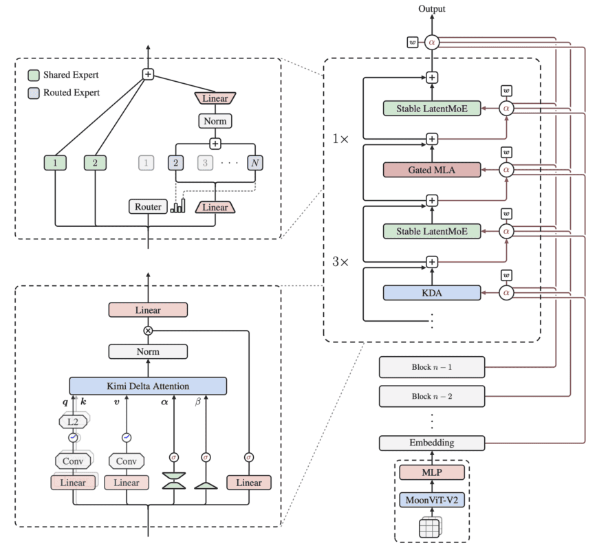
The logic of the architecture is organized around three dimensions along which information travels inside the model: sequence length, network depth, and layer width. Each dimension gets its own component.
Sequence length: hybrid KDA and Gated MLA attention
Ordinary softmax attention is quadratic in sequence length, which is unworkable at a million tokens. Kimi K3 alternates two mechanisms in a 3:1 ratio. Three consecutive layers use Kimi Delta Attention (KDA), linear attention with a fixed-size recurrent state, and the fourth is Gated MLA, full global attention with a compressed KV cache.
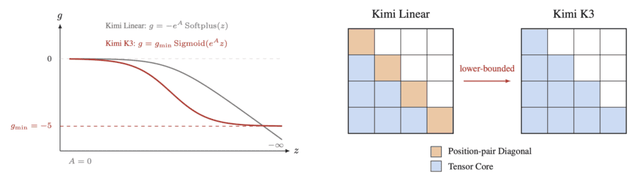
KDA works by a delta rule: the state is updated as a combination of forgetting old content and writing new content. The key parameter here is the retention factor, which Kimi K3 bounds from below. It sounds like a detail, but the consequences are purely engineering. In the previous version (Kimi Linear) the factor could drift arbitrarily close to zero, and its reciprocal in the rescaling step grew beyond the range of BF16. Because of that, diagonal tiles had to be computed along a separate slow path. By bounding the log-decay from below at −5, the authors fit the whole range into BF16 and moved every tile onto dense matrix multiplications on Tensor Cores.
Another consequence of the hybrid: no positional encoding is used at all (NoPE). Information about token order is carried by KDA’s recurrent decay, while the MLA layers provide unrestricted global interaction by content. This is why Kimi K3 extrapolates to a million tokens without retuning the RoPE frequency base and without YaRN.
Depth: Attention Residuals
In a standard transformer, residual connections compress all prior information into a single state passed down through depth. That is a bottleneck, much like the one RNNs suffered from over time. Attention Residuals (AttnRes) apply to depth the same idea that attention used to fix RNNs: each layer decides for itself what to pull from which preceding layers, through a learnable pseudo-query and softmax weights over the outputs of all earlier layers.
The full version costs O(L²d) arithmetic, which is tolerable at fewer than 100 layers, but it requires keeping every layer’s output in memory. So the layers are partitioned into blocks: inside a block the outputs are summed into a single representation, and attention across depth runs only between blocks. Overhead drops from O(Ld) to O(Nd). In Kimi K3 that means 8 blocks of 12 layers.
Width: Stable LatentMoE and Quantile Balancing
A conventional MoE sends each selected expert the full d-dimensional token representation, so traffic grows linearly with the number of active experts. LatentMoE separates model width from expert width: shared experts operate at full width, while the specialized routed experts live in a compact latent space. That made it possible to scale to 896 routed experts with 16 active per token, a sparsity of 56.
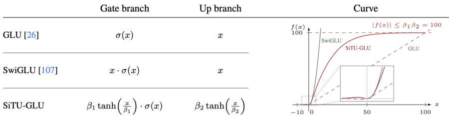
This level of sparsity breaks two things. First, the routed path chains nearly four consecutive matrix multiplications, and at 2.8 trillion parameters the activations start to blow up. The fix is an RMSNorm before the up-projection plus a new activation, SiTU-GLU, which softly caps both GLU branches through a scaled tanh. Near zero it almost coincides with SwiGLU, while for large positive inputs it saturates at a ceiling of 100.
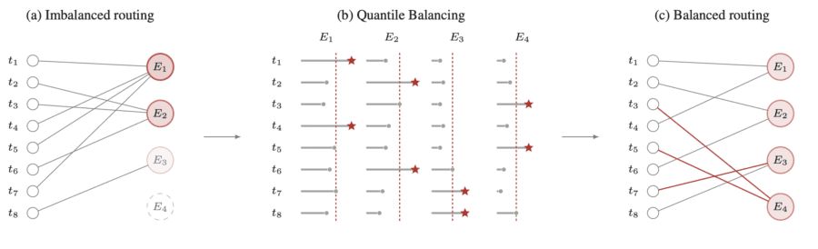
The second problem: balancing the load across nearly a thousand experts no longer works the old way. The standard approach adds a per-expert bias to the router score and nudges it by a fixed step toward whichever side is underloaded. The step has to be tuned by hand: small means slow adaptation, large means the load oscillates.
Quantile Balancing (QB) solves it differently. Instead of stepping in the right direction, the bias is set directly to the point where the expert receives exactly its target load, and that point turns out to be a quantile of the distribution of score margins across tokens. No learning-rate-like hyperparameter is needed, and equilibrium is reached within a few steps. Computing an exact quantile over millions of tokens spread across nodes is impossible, so each expert keeps a histogram: one all-reduce of integer counters per step, and the quantile is recovered from the pooled bins up to the bin width.
How Kimi K3 handles images
Here the authors depart from common practice. The vision encoder is usually initialized from a contrastively pre-trained model such as SigLIP, on the assumption that ready-made visual features give the model a head start. In Kimi K3 the MoonViT-V2 encoder was trained from scratch on plain next-token prediction, and the main reason is training stability.
When a pre-trained encoder is attached to the language model, joint optimization behaves badly: the SigLIP-initialized variant shows consistently higher gradient norms with constant spikes. Training from scratch runs smoothly. Meanwhile, on vision benchmarks MoonViT-V2 matches the SigLIP-initialized baseline, from which the authors conclude that contrastive pre-training is simply unnecessary as an initialization for multimodal models at scale.
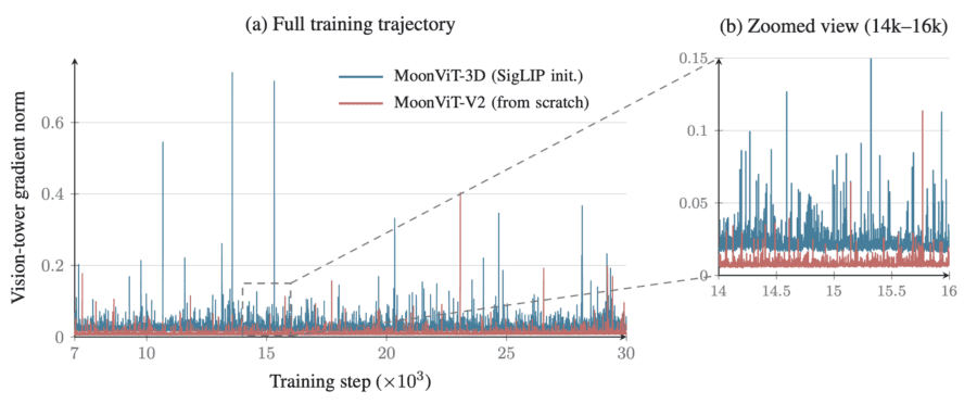
The encoder itself is a 27-layer vision transformer with roughly 0.4 billion parameters and no bias terms. Before projection into the language model, a pixel-shuffle with 2×2 downsampling cuts the number of visual tokens fourfold, which makes images up to 3584×3584 pixels affordable inside the context.
Scaling law: a 2.5× gain over Kimi K2
Architectural changes also change the optimal training regime, so batch size, learning rate, tokens-per-parameter ratio and model shape were all retuned for Kimi K3. Measured on held-out validation data, the combined gain in scaling efficiency came to roughly 2.5× over Kimi K2. In other words, Kimi K3 reaches the same validation loss with about 2.5 times fewer FLOPs.
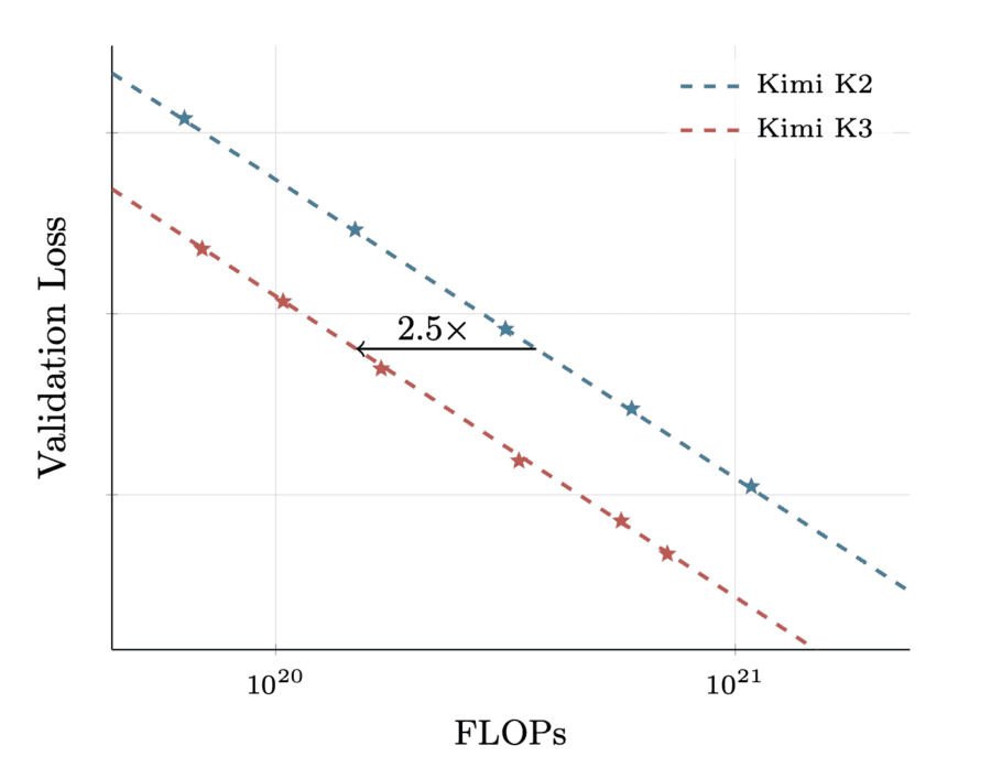
One separate observation about the learning rate schedule: cosine decay consistently beats warmup stable decay. The authors underline a methodological point here. The two schedules have markedly different optimal hyperparameters even at the same model size and token budget, so comparing them on a shared set of hyperparameters is unfair: whichever schedule those hyperparameters suit better will win. Here a separate search was run for each schedule, and cosine decay still produced a lower final loss.
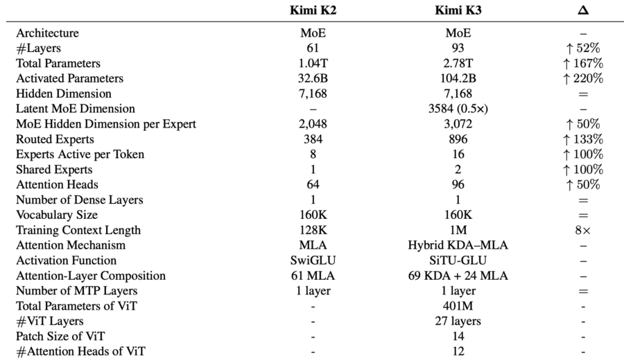
The architecture comparison table shows the concrete changes: 93 layers instead of 61, 896 routed experts instead of 384, 16 active experts per token instead of 8, 96 attention heads instead of 64, and a training context that grew from 128K to 1M. The hidden dimension stayed the same at 7,168.
The context window was grown gradually, over four stages: from 8K to 64K during pre-training, and from 256K to 1M during cooldown. Concentrating the expensive long-sequence computation in a small share of the total budget keeps the curriculum economical. One further detail: length alone is not treated as a sufficient signal, so long-context data is also synthesized by permuting and concatenating documents and sub-tasks, so that a task can only be solved by gathering information scattered across the full million tokens. Otherwise attention degenerates into local patterns.
Post-training: nine teachers in one student
The pipeline after pre-training has three stages.
First comes SFT, assembling a large instruction dataset weighted toward complex agentic trajectories. The trajectories are synthesized by domain-specialized models from earlier Kimi generations, then run through multi-stage verification and human-in-the-loop annotation.
Next is RL, but not one model per task. Reinforcement learning is scaled across three broad domains (general tasks, general agents, coding agents) and three levels of reasoning effort (low, high, max). Crossed together, that yields nine expert models. Effort levels are enforced through a token budget: each problem gets an initial budget, and any trajectory that exceeds it receives a reward of −1. A large-budget variant is trained first, then the multiplier is annealed downward to obtain the more economical variants.
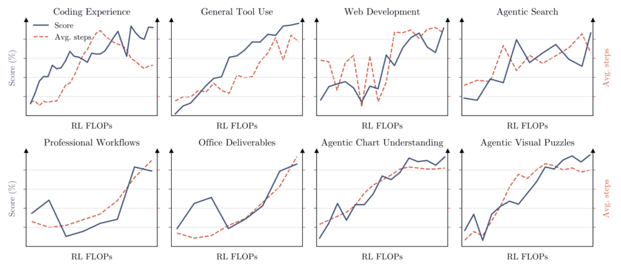
The third stage consolidates the nine experts into one model through Multi-Teacher On-Policy Distillation. The student generates its own responses, and the per-token reward is a clipped log ratio of the teacher’s and the student’s probabilities. The teacher is selected by domain and effort level. This dense signal plugs directly into the RL framework and inherits the same infrastructure optimizations.
RL tasks are not only taken off the shelf. They are synthesized from a knowledge graph that agents expand themselves through web search, running from broad domains (mathematics, chemistry, the humanities) down to narrow concepts such as RoPE or GPU kernels. A keyword set is assembled from the sampled nodes, real materials are retrieved with it (papers, blog posts, repositories), and a task is synthesized from those materials.
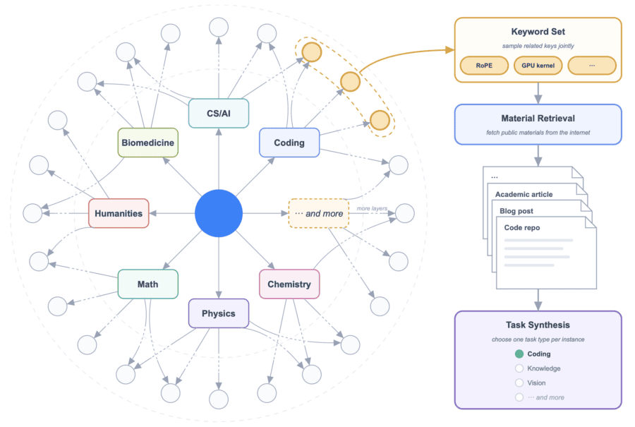
Autonomous Execution Tasks deserve a separate mention: the agent sees only the objective, the context, the constraints and the verification interface, with no reference trajectories or predefined procedures. Reward is grounded in the final state of the environment rather than in the agent’s own report of completion. Reward hacking is suppressed by separating a public verifier that gives diagnostic feedback from a hidden verifier that evaluates held-out scenarios.
Training and inference infrastructure
The infrastructure section takes up more room in the Kimi K3 report than the architecture and post-training sections combined, which is telling in itself.
MoonEP was built for training a MoE at 2.8 trillion parameters. The idea is that every rank receives exactly the same number of tokens, which is achieved by duplicating some experts. The authors prove that a balanced plan always exists with at most E/R redundant experts per rank (E being the number of experts, R the group size), and that this bound is essentially tight. The practical payoff is that the planner never hits a dead end and training never has to stop, whereas earlier solutions set the cap manually and broke whenever no plan fit inside it. Perfect balance also makes computation shapes statically known, which removes host-device synchronization at every layer.
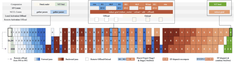
For agentic RL at million-token contexts, the team wrote AgentENV, a sandbox environment on isolated Firecracker microVMs. The reason is not only security: conventional container-based sandboxes produced kernel panics and deadlocks under aggressive agent behavior. Incremental checkpoints save only the memory pages dirtied since the last one, giving latencies of 133 ms to checkpoint and 49 ms to resume. A paused sandbox consumes no resources, and it can spend up to 98% of its lifetime waiting on the model’s response. Across all of Kimi K3’s training and evaluation, 51,219,741 sandboxes were created across 1,505,678 images.
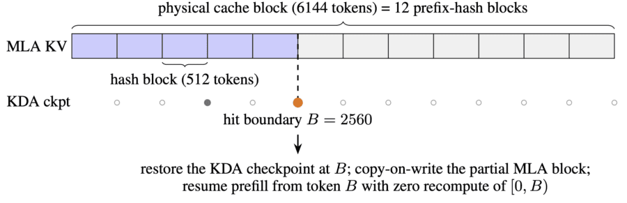
Inference is complicated further by the hybrid architecture maintaining two fundamentally different caches. The MLA KV cache grows with length and is paged per token, while the KDA recurrent state is fixed in size with a single copy per request. Naively merging them forces a shared block size of 1,024 to 6,144 tokens, at which prefix caching becomes nearly useless: requests shorter than one block can never be reused at all. The solution is to decouple the granularities: prefix hashing runs on fine 512-token blocks, while KDA state checkpoints are saved only at a sparse subset of those boundaries, typically at conversation-turn boundaries.
One more practically useful detail: the MoE expert weights, which dominate memory, are quantized to MXFP4 with activations computed in MXFP8, while everything else stays at higher precision. Quantization is accounted for throughout post-training (QAT), and during RL the rollout and the training share the same quantization scheme, which removes the train-inference mismatch.
Kimi K3 benchmark results
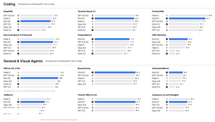
The overall picture: Kimi K3 trails the two strongest proprietary models (Claude Fable 5 and GPT-5.6 Sol) by a modest margin and consistently leads everything else, including Claude Opus 4.8, GPT-5.5 and the open GLM-5.2.
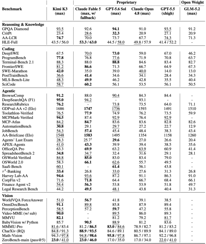
On reasoning and knowledge the model is at frontier level on GPQA Diamond (93.5%), but it falls noticeably behind on research-level tasks: HLE-Full at 43.5% without tools and 56.0% with them, CritPt at only 23.4%. The authors name research-level reasoning outright as the main area for improvement.
In coding, the best score goes to ProgramBench (77.8%) and SWE-Marathon (42.0%, 7 points ahead of Claude Fable 5, and this is a GPU-kernel optimization suite). On Terminal-Bench 2.1 it nearly ties GPT-5.6 Sol (88.3% versus 88.8%). On FrontierSWE it takes second place with 81.2%.
Agentic tasks are where Kimi K3 collects the most first places: BrowseComp 91.2%, DeepSearchQA 95.0 F1, MCPMark-Verified 94.5%, Harvey Lab-AA 94.6%. It slips mainly on the Elo-rated suites that judge the quality of knowledge work: third on GDPval-AA v2 and second on AA-Briefcase.
Independent evaluations put it fourth of 580 models on Artificial Analysis’s Intelligence Index v4.1 (57.1) and second of 39 on the Vals AI index (74.7%). WebDev Arena deserves a separate note: Kimi K3 ranks first of 99 models with 1,678 Elo and became the first open model to top that leaderboard.
What Kimi K3 inference costs
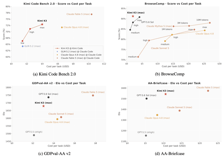
The cost side is no less interesting than the scores. On Kimi Code Bench 2.0 the model is 4 points behind Claude Fable 5 but runs at 38% of its cost, and at high effort it already matches Claude Opus 4.8’s maximum-effort score at roughly a third of the price. On BrowseComp the top score (91.2%) comes in at $2.03 per task, half the cost of GPT-5.6 Sol and an order of magnitude below the Claude models at maximum effort.
Cybersecurity: what an open-weights model can do
This section is worth attention if only because open weights leave no way to restrict anything after the fact. The evaluation ran across two tiers of risk.
At the first tier (vulnerability discovery and proof-of-concept work) Kimi K3 went through dozens of widely deployed products: OS kernels, databases, web frameworks, blockchain, VPN software. Of the findings that reached human review, roughly 70% were confirmed as genuine, including 16 previously unknown vulnerabilities across six projects. Two findings in the Linux kernel were confirmed by security experts as a remote denial-of-service primitive and as a deterministic local privilege-escalation primitive.
At the second tier (writing a working end-to-end exploit) the model solved 14 of 36 tasks against 8 of 36 for GLM-5.2. The successes are unevenly distributed: 10 of the 14 come from the user-space track, while on the kernel track neither model solves three quarters of the tasks. Every task in the suite is solvable by humans, and the full suite is estimated at roughly 540 expert-hours. An independent joint assessment by the UK AI Security Institute and NIST CAISI reached the same conclusions: Kimi K3 outperforms GLM-5.2, but on completed exploitation chains it trails the frontier proprietary models, achieving arbitrary code execution on 0 of 41 tasks.
One more detail from the report: frontier models from Anthropic and OpenAI refuse cyber-related tasks, which made a comparable evaluation impossible, so they were excluded from this suite.
What Kimi K3 has already done on its own
The section on applied cases is more convincing than abstract percentages.
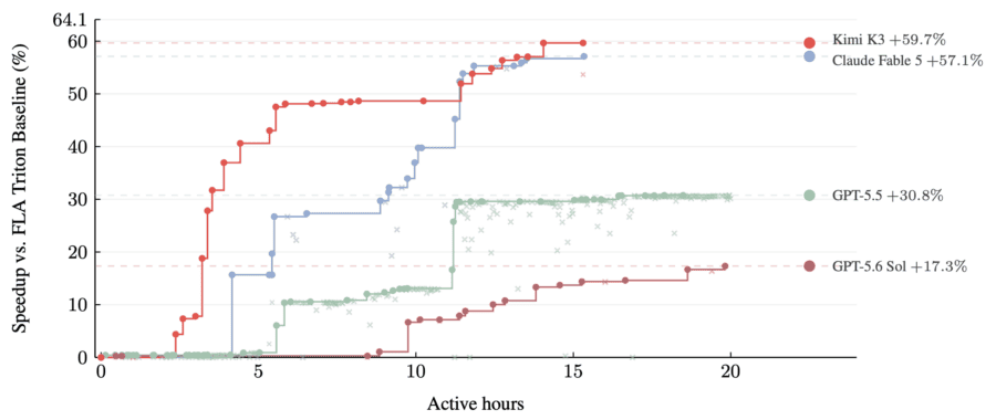
GPU kernel optimization: the model cut AttnRes kernel latency from 283.6 ms to 114.4 ms, reduced DSA and KDA runtime by 55.1% and 73.6% respectively, and pushed past half of peak TFLOPS on MLA. The authors note separately that an early Kimi K3 checkpoint was already handling most of their own kernel optimization work during late-stage development.
The MiniTriton compiler: a compact Triton-like system with its own Python frontend, an MLIR annotation layer and PTX code generation. Its from-scratch tensor-core matmul approaches cuBLAS at the largest shapes (about 90% of the measured machine roof), and training a GPT model on it produces a loss curve tracking the PyTorch reference, with gradients differing by no more than torch’s own fp32 rounding error.
Chip design: in a single autonomous 48-hour run, Kimi K3 built, optimized and verified a prototype inference chip using open-source EDA tools. Within a 4 mm² area budget the design closes timing at 100 MHz and delivers over 8,700 tokens per second in RTL simulation.
There are cases of a different kind too: reproducing the I–Love–Q universal relations in computational astrophysics (over 20 papers reviewed, more than 300 equations of state evaluated, 3,000+ lines of Python and an interactive dashboard, in about two hours against one to two weeks for an experienced researcher), and editing a video from 56 source clips with frame-accurate beat synchronization.
Why the comparison numbers come with caveats
A few caveats worth keeping in mind when reading the Kimi K3 figures.
Claude Fable 5’s results in the comparison tables were obtained with fallback behaviors enabled, and GPT-5.6 Sol’s include potential cyberguards, which the authors state plainly in the footnotes. On some in-house suites Claude Fable 5 refused a noticeable share of tasks (14 tasks in Online Experience, and 13 fallbacks out of 80 on Kimi Code Bench 2.0), which directly affects comparability.
Some results are taken from third-party leaderboards on a specific date, and Elo scores drift as more matches accumulate. The authors themselves call the cyber evaluation a lower bound on capability and promise to revisit it at every major model update.
And the main limitation stays the same as with its predecessors: 2.8 trillion parameters is not a model you deploy on a couple of cards. Open Kimi K3 weights matter mostly as a foundation for research, distillation, and for those who already have the hardware fleet, rather than as something you run locally.