Methods that reconstruct 3D models of people’s heads from images need to account for varying 3D pose, lighting, non-rigid changes due to expressions, relatively smooth surfaces of faces, ears, and neck, and finally, the hair. Great reconstructions can be achieved nowadays in case the input photos are captured in a calibrated lab setting or semi-calibrated setup where the person has to participate in the capturing session (see related work).
Reconstructing from Internet photos, however, is an open problem due to the high degree of variability across uncalibrated images. Lighting, pose, cameras and resolution change dramatically across photos. In recent years, reconstruction of faces from the Internet has received a lot of attention. All face-focused methods, however, mask out the head using a fixed face mask and focus only on the face area.
Previous Works
Calibrated head modeling has achieved amazing results over the last decade. Reconstruction of people from Internet photos recently achieved good results.
- Shlizerman et al. showed that it is possible to reconstruct a face from a single Internet photo using a template model of a different person. One way to approach the uncalibrated head reconstruction problem is to use the morphable model approach.
- Hsieh et al. showed that with morphable models the face is fitted to a linear space of 200 face scans, and the head is reconstructed from the linear space as well. In practice, morphable model methods work well for face tracking.
- Adobe Research proved that hair modeling could be done from a single photo by fitting to a database of synthetic hairs or by fitting helices.
State-of-the-art idea
This idea addresses the new direction of head reconstruction directly from Internet data. Given a photo collection, obtained by searching for photos of a specific person on Google image search, the task is to reconstruct a 3D model of that person’s head(the focus is only on the face area). If the given photos are only one or two per view, the problem is very challenging due to lighting inconsistency across views, difficulty in segmenting the face profile from the background, and challenges in merging the images across views. The key idea is that with many more (hundreds) of photos per 3D view, the problems can be overcome. For celebrities, one can quickly acquire such collections from the Internet; for others, we can extract such photos from Facebook or mobile photos.
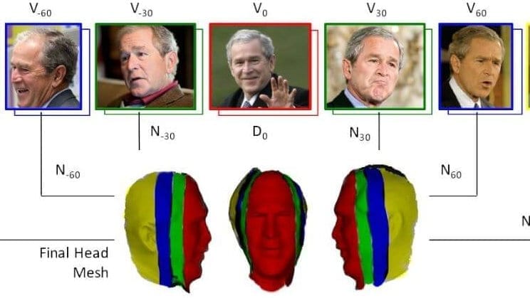
The method works as follows: a person’s photo collection is divided into clusters of approximately the same azimuth angle of the 3D pose. Given the clusters, a depth map of the frontal face is reconstructed, and the method gradually grows the reconstruction by estimating surface normals per view cluster and then constraining using boundary conditions coming from neighboring views. The final result is a head mesh of the person that combines all the views.
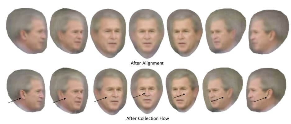
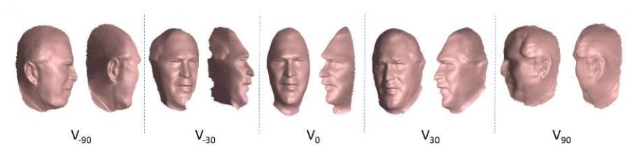
The given photos are divided into a view cluster as Vi. Photos in the same view cluster have approximately the same 3D pose and azimuth angle. The photos with 7 clusters with azimuths: i= 0,−30,30,−60,60,−90,90. Figure 2 shows the averages of each cluster after rigid alignment using fiducial points (1st row) and after subsequent alignment using the Collection Flow method (2nd row), which calculates optical flow for each cluster photo to the cluster average.
Head Mesh Initialization
The goal is to reconstruct the head mesh M. It starts with estimating a depth map and surface normals of the frontal cluster V0, and assign each reconstructed pixel to a vertex of the mesh. The algorithm is as follows:
- Dense 2D alignment: Photos are first rigidly aligned using 2D fiducial points as the pipeline. The head region including neck and shoulder in each image is segmented using semantic segmentation. Then Collection Flow is run on all the photos in V0 to align them with the average photo of that set densely. The challenging photos do not affect the method; given that the majority of the images are segmented well, Collection Flow will correct for inconsistencies. Also, Collection Flow helps to overcome differences in hairstyle by warping all the photos to the dominant style.
- Surface normals estimation: A template face mask is used to find the face region on all the photos. Photometric Stereo (PS) is then applied to the face region of the flow-aligned photos. The face region of the images are arranged in a n×pk matrix Q, where n is the number of pictures and pk is the number of face pixels determined by the template facial mask. Rank-4 PCA is computed to factorize into lighting and normals: Q=LN. After getting the lighting estimation L for each photo, calculate N for all p head pixels including ear, chin and hair regions. Two key components that made PS work on uncalibrated head photos are:
- Resolving the Generalized Bas-Relief (GBR) ambiguity using a template 3D face of a different individual.
- Using a per-pixel surface normal estimation, where each point uses a different subset of photos to estimate the normal.
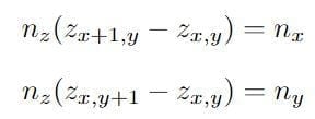
- Depth map estimation: The surface normals are integrated to create a depth map Do by solving a linear system of equations that satisfy gradient constrains dz/dx=−nx/ny and dz/dy=−nx/ny where (nx,ny,nz) are components of the surface normal of each point. Combining these constraints, for the z-value on the depth map:
 This generates a sparse matrix of 2p×2p matrix M, and solve for:
 This generates a sparse matrix of 2p×2p matrix M, and solve for:
Boundary-Value Growing
To complete the side view of Mesh, boundary value growing is introduced. Starting from the frontal view mesh V0, we gradually complete more regions of the head in the order of V30, V60, V90 and V−30, V−60, V−90 with two additional key constraints.
- Ambiguity recovery: Rather than recovering the ambiguity A that arises from Q=LA^(−1)AN using the template model, already computed neighboring cluster is used, i.e., for V±30, N(zero) is used, for V±60, N±30 is used, and for V±90, N±60 is used. Specifically, it estimates the out-of-plane pose from the 3D initial mesh V0 to the average image of pose cluster V30.
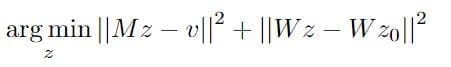
- Depth constraint: In addition to the gradient constraints, boundary constraints are also modified. Let Ω0 be the boundary of D′0. Then the part of Ω0 that intersects the mask of D30 will have the same depth values: D30(Ω0) =D′0(Ω0). With both boundary constraints and gradient constraints, the optimization function can be written as:
After each depth stage reconstruction (0,30,60,.. degrees), the estimated depth is projected to the head mesh. By this process, the head is gradually filled in by gathering vertices from all the views.
Result
Below fig shows the reconstruction per view that was later combined to a single mesh. For example, the ear in 90 and -90 views is reconstructed well, while the other views are not able to reconstruct the ear.
In Figure 5, it is shown how two key constraints work well in the degree 90 view reconstruction result. Without the correct reference normals and depth constraint, the reconstructed shape is flat, and the profile facial region is blurred, which increased the difficulty of aligning it back to the frontal view.
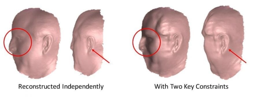
The left two shapes show the two views of 90-degree view shape reconstructed independently without two key constraints. The right two shapes show the two views of the result with two key constraints. Figure 6 shows the reconstruction result for 4 subjects; each mesh is rotated to five different perspectives.
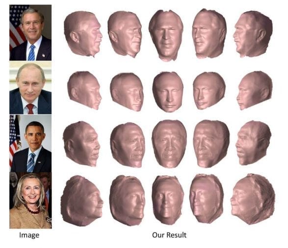
Fig:6 Final reconstructed mesh rotated to 5 views to show the reconstruction from all sides. Each color image is an example image among around 1,000 photo collection for each person.
Comparison with other models
In Figure 6 a comparison is shown to the software FaceGen that implements a morphable model approach.
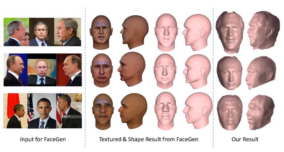
Figure 6
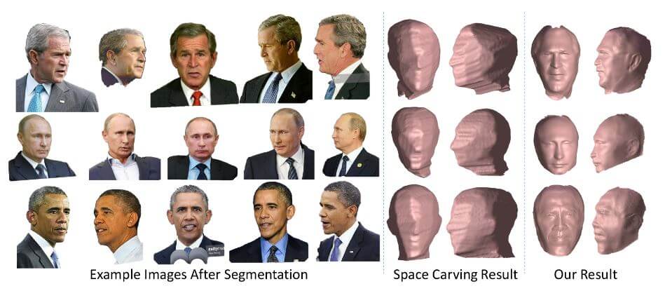
For a quantitative comparison, for each person, the reprojection error is calculated of the shapes from three methods (suggested approach, Space Carving and FaceGen) to 600 photos in different poses and lighting variations. The 3D shape comes from each reconstruction method.
The average reprojection error is shown in below Table.
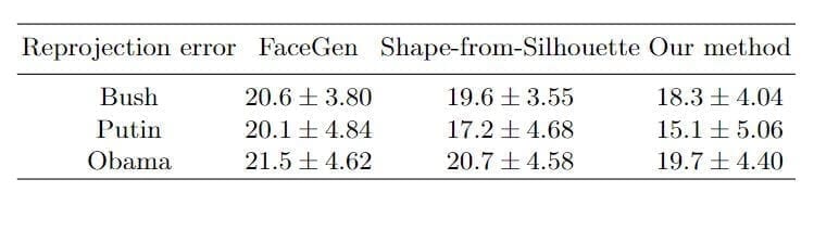
Reprojection error from 3 reconstruction methods
The error map of an example image is shown in Figure 7. Notice that the shapes from FaceGen and Space Carving might look good from the frontal view, but they are not correct when rotating to the target view. See how different the ear part is in the figure.
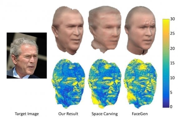
Figure 7: Visualisation of the re-projection error for 3 methods
Conclusion
This approach shows that it is possible to reconstruct head from internet photos. However, this approach has the number of limitations. First, it assumes a Lambertian model for surface reflectance. While this works well, accounting for specularities should improve results. Second, fiducials for side views were labeled manually. Third, the complete model is not constructed; the top of the head is missing. To solve this more photos need to be added with different elevation angles, rather than just focusing on the azimuth change.