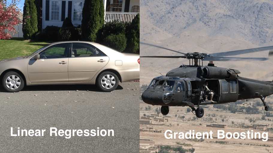
Gradient boosting is a machine learning technique that builds a strong model from many weak ones, usually small decision trees, by adding them one at a time. Each new tree is trained to correct the errors that the current ensemble still makes — technically, to follow the negative gradient of the loss function. Gradient boosted trees, in implementations such as XGBoost, LightGBM and CatBoost, are the most accurate general-purpose models for tabular data and have won a large share of Kaggle competitions.
This guide explains the intuition behind gradient boosting, walks through the algorithm step by step, shows how it relates to gradient descent, compares it with random forests and AdaBoost, and gives working Python code: a from-scratch implementation and a comparison of XGBoost, LightGBM and scikit-learn.
Key takeaways
- Idea: start with a simple prediction, then repeatedly add a small tree that predicts what the model still gets wrong.
- For squared error, “what the model gets wrong” is simply the residuals
y − ŷ; for other losses it is the negative gradient. - Boosting builds trees sequentially to reduce bias; bagging and random forests build them independently to reduce variance.
- The key hyperparameters are the learning rate, the number of trees and tree depth. Use early stopping to choose the number of trees.
- In practice use XGBoost, LightGBM, CatBoost or scikit-learn’s HistGradientBoosting rather than writing your own.
What Is Gradient Boosting?
A single decision tree is easy to understand but rarely accurate: a shallow tree is too simple and underfits, a deep tree memorizes the training data and overfits. Gradient boosting gets around this by combining hundreds or thousands of shallow trees. None of them is good on its own — each is a weak learner, only slightly better than guessing — but together they form a very flexible model.
The trees are not trained independently. Each one is fitted to the mistakes of all the trees before it, and its prediction is added to the running total with a small weight. The final model is a sum:
F(x) = F₀(x) + η · h₁(x) + η · h₂(x) + … + η · hM(x)
Here F₀ is the initial guess (for regression, the mean of the target), each hₘ is a small tree, M is the number of trees and η is the learning rate. The method was formalized by Jerome Friedman in 1999–2001 under the name gradient boosting machine (GBM); you will also see it called GBDT (gradient boosted decision trees) or gradient boosted trees. It works for regression, classification and ranking.
Ensembles: Bagging vs Boosting
An ensemble combines several models so that their errors partly cancel out. Prediction errors come from three sources: noise in the data, which no model can remove; bias, when the model is too simple to capture the pattern; and variance, when the model is so sensitive to the training data that it changes a lot from sample to sample. The two main ensemble strategies attack different parts of this.
- Bagging (bootstrap aggregating) trains many models independently, each on a random resample of the data, and averages their predictions. Averaging many noisy but unbiased models reduces variance. Random forest is the best-known example: deep trees, each trained on a bootstrap sample and a random subset of features.
- Boosting trains models sequentially. Each model focuses on the examples that the previous ones handled badly. Starting from simple, high-bias models and correcting them step by step reduces bias. AdaBoost does this by reweighting misclassified examples; gradient boosting does it by fitting each new model to the gradient of the loss.
Because boosting keeps reducing training error, it can overfit if it runs too long. That is why the number of trees has to be controlled, usually with a validation set.
The Intuition: Learning From Residuals
A residual is the difference between the true value and the prediction, y − ŷ. If a model has captured all the structure in the data, its residuals look like random noise scattered around zero, with no pattern left to exploit:
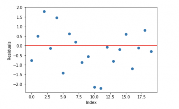
If the residuals do have a pattern — say, the model is consistently too low for one range of inputs — then that pattern is information the model has missed. Gradient boosting turns this observation into an algorithm: train a new model to predict the residuals, add its predictions to the old ones, and look at the residuals again. Repeat until they stop showing a pattern. In plain steps:
- Fit a simple model to the data.
- Compute the residuals: where and by how much the model is wrong.
- Fit a new small model that predicts those residuals from the same inputs.
- Add a fraction of its predictions to the current model.
- Repeat steps 2–4, stopping when validation error no longer improves.
The Gradient Boosting Algorithm
For a differentiable loss function L(y, F(x)) and n training examples, the general algorithm is:
- Initialize with the constant that minimizes the loss:
F₀(x) = argminc Σ L(yᵢ, c). For squared error this is the mean ofy; for log-loss it is the log-odds of the positive class. - For m = 1 to M:
- compute the pseudo-residuals, the negative gradient of the loss with respect to the current predictions:
rᵢ = −∂L(yᵢ, F(xᵢ)) / ∂F(xᵢ); - fit a regression tree
hₘto the pairs(xᵢ, rᵢ); - update the model:
Fₘ(x) = Fₘ₋₁(x) + η · hₘ(x).
- compute the pseudo-residuals, the negative gradient of the loss with respect to the current predictions:
- Output
FM(x).
For mean squared error, L = ½(y − F)², the negative gradient is exactly y − F: the pseudo-residuals are the ordinary residuals, and the algorithm is the intuitive “fit the errors” loop from the previous section. For classification with log-loss, the pseudo-residuals are y − p, the difference between the label and the predicted probability. Practical implementations also recompute the value in each leaf of the tree to minimize the loss exactly, which matters for losses other than squared error.
Step-by-Step Example
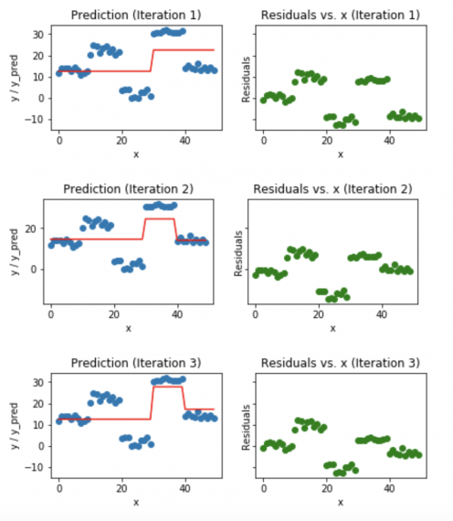
Take a toy regression problem with one input x from 0 to 49 and a target that jumps between five levels:
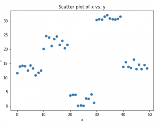
Use decision stumps — trees with a single split — as weak learners. The first stump can only split the data into two groups, so its prediction (red line, left) is a crude step, and the residuals (green, right) still show the original structure clearly. The second stump is trained on those residuals and adds another split; the third adds another:
After enough iterations the prediction follows every level of the data and the residuals are just noise around zero, so there is nothing more to learn. Continuing past this point would start fitting the noise:
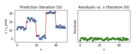
The Python implementation of exactly this loop is shown below.
Why It Is Called Gradient Boosting
In gradient descent, you minimize a loss by moving the parameters a small step against the gradient: θ ← θ − η · ∇L. Gradient boosting does the same thing, but in the space of predictions. The current predictions F(xᵢ) play the role of the parameters, the negative gradient tells you which direction would reduce the loss for each training example, and a tree is fitted to that direction so the step generalizes to new inputs. The learning rate η is the step size.
This view is what makes gradient boosting so general. Any differentiable loss works: squared error or Huber loss for regression, log-loss for classification, ranking losses for search. You only change how the pseudo-residuals are computed; the rest of the algorithm stays the same.
Key Hyperparameters
| Hyperparameter | What it controls | Typical values | Names in libraries |
|---|---|---|---|
| Number of trees | How many boosting rounds | 100–5,000, set by early stopping | n_estimators, num_boost_round, max_iter |
| Learning rate | How much each tree contributes | 0.01–0.3 | learning_rate, eta |
| Tree depth or leaves | How complex each tree is | depth 3–8, or 15–255 leaves | max_depth, num_leaves, max_leaf_nodes |
| Row subsampling | Fraction of rows used per tree | 0.5–1.0 | subsample, bagging_fraction |
| Column subsampling | Fraction of features used per tree | 0.5–1.0 | colsample_bytree, feature_fraction |
| Minimum leaf size | Smallest allowed leaf | 1–100 examples | min_child_weight, min_data_in_leaf, min_samples_leaf |
| Regularization | Penalty on leaf values | 0–10 | reg_lambda, reg_alpha, l2_regularization |
The learning rate and the number of trees trade off against each other: halving the learning rate roughly doubles the number of trees needed, usually with slightly better accuracy. A reliable recipe is to fix a small learning rate such as 0.05, set the number of trees to a large upper bound, and let early stopping on a validation set pick the actual number. Using a random fraction of rows for each tree is called stochastic gradient boosting; it speeds up training and usually reduces overfitting.
XGBoost vs LightGBM vs CatBoost
Modern libraries implement the same core algorithm with engineering that makes it far faster and more robust than the original GBM.
| Library | Released | Distinctive features | Good fit |
|---|---|---|---|
| XGBoost | 2014 | Regularized objective with L1/L2 on leaf weights, second-order gradients, sparse-aware splits, GPU and distributed training | Strong default, very mature ecosystem |
| LightGBM | 2016 (Microsoft) | Histogram-based splits, leaf-wise tree growth, gradient-based sampling (GOSS), very fast on large data | Large datasets, fast iteration |
| CatBoost | 2017 (Yandex) | Native categorical features with ordered target statistics, symmetric trees, good results with default settings | Data with many categorical columns |
| scikit-learn HistGradientBoosting | 2019 | LightGBM-style histogram algorithm, native missing values and categorical support, no extra dependency | Projects already built on scikit-learn |
On most problems the accuracy differences between them are small once each is tuned; speed, categorical handling and the rest of your stack usually decide. Avoid scikit-learn’s older GradientBoostingRegressor and GradientBoostingClassifier for anything beyond small datasets — they are exact but much slower than the histogram-based estimators.
Gradient Boosting vs Random Forest vs AdaBoost
| Random forest | AdaBoost | Gradient boosting | |
|---|---|---|---|
| Ensemble type | Bagging | Boosting | Boosting |
| Trees trained | Independently, in parallel | Sequentially | Sequentially |
| Typical trees | Deep, low bias | Stumps | Shallow, 3–8 levels |
| How errors are corrected | Averaging | Reweighting misclassified examples | Fitting the negative gradient of the loss |
| Main effect | Reduces variance | Reduces bias | Reduces bias |
| Tuning effort | Low | Low | Moderate |
| Overfitting risk | Low | Moderate, sensitive to noise | Moderate, controlled by early stopping |
| Accuracy on tabular data | Good | Fair | Usually best |
AdaBoost turns out to be a special case of gradient boosting with an exponential loss. Random forests remain a great baseline: they need almost no tuning and are hard to overfit. When you have time to tune, gradient boosting usually wins.
Gradient Boosting in Python
From scratch
The loop below is the whole algorithm for squared error: start from the mean, compute residuals, fit a decision stump to them, add a fraction of its prediction, repeat. It uses data shaped like the example above:
import numpy as np
from sklearn.tree import DecisionTreeRegressor

# Step-shaped data: 50 points, five flat regions plus noise
rng = np.random.default_rng(42)
x = np.arange(50).reshape(-1, 1)
levels = [13, 22, 2, 31, 14]
y = np.repeat(levels, 10) + rng.normal(0, 1.5, 50)

def gradient_boosting(x, y, n_trees=50, learning_rate=0.5, max_depth=1):
    f0 = y.mean()                       # step 0: predict the mean
    pred = np.full(len(y), f0)
    trees = []
    for m in range(n_trees):
        residuals = y - pred            # negative gradient of squared error
        tree = DecisionTreeRegressor(max_depth=max_depth)
        tree.fit(x, residuals)          # fit a weak learner to the residuals
        pred += learning_rate * tree.predict(x)
        trees.append(tree)
        if m in (0, 1, 2, 9, 49):
            print(f"after {m + 1:>2} trees: MSE = {np.mean((y - pred) ** 2):.2f}")
    return f0, trees

f0, trees = gradient_boosting(x, y)
Output:
after  1 trees: MSE = 76.55
after  2 trees: MSE = 71.45
after  3 trees: MSE = 63.00
after 10 trees: MSE = 31.62
after 50 trees: MSE = 1.90
The training error falls from the variance of the data, about 96, to 1.9 — close to the noise level of 2.25 that was added on purpose. A real implementation would also need prediction on new data and early stopping, but the learning loop is exactly this.
XGBoost, LightGBM and scikit-learn
All the main libraries share the familiar scikit-learn interface. Here they are on Friedman #1, a standard nonlinear regression benchmark built into scikit-learn, with a random forest for reference:
from sklearn.datasets import make_friedman1
from sklearn.model_selection import train_test_split
from sklearn.metrics import mean_squared_error
from sklearn.ensemble import RandomForestRegressor, HistGradientBoostingRegressor
from xgboost import XGBRegressor
from lightgbm import LGBMRegressor

# Nonlinear benchmark: y depends on 5 of 10 features, plus noise
X, y = make_friedman1(n_samples=20_000, n_features=10, noise=1.0, random_state=0)
X_train, X_test, y_train, y_test = train_test_split(X, y, test_size=0.2, random_state=0)

models = {
    "Random forest": RandomForestRegressor(n_estimators=300, n_jobs=-1, random_state=0),
    "sklearn HistGB": HistGradientBoostingRegressor(max_iter=500, learning_rate=0.1, random_state=0),
    "XGBoost": XGBRegressor(n_estimators=500, learning_rate=0.1, max_depth=4, random_state=0),
    "LightGBM": LGBMRegressor(n_estimators=500, learning_rate=0.1, num_leaves=15, random_state=0, verbose=-1),
}
for name, model in models.items():
    model.fit(X_train, y_train)
    rmse = mean_squared_error(y_test, model.predict(X_test)) ** 0.5
    print(f"{name:>14}: test RMSE = {rmse:.3f}")
Output (scikit-learn 1.9, XGBoost 3.4, LightGBM 4.7):
 Random forest: test RMSE = 1.396
sklearn HistGB: test RMSE = 1.109
       XGBoost: test RMSE = 1.076
      LightGBM: test RMSE = 1.093
The noise in this dataset has a standard deviation of 1.0, so no model can get below an RMSE of about 1. All three boosting libraries come close; the random forest is noticeably behind.
Early stopping
Instead of guessing the number of trees, give the model a large upper bound and a validation set, and let it stop when the validation error stops improving:
from sklearn.datasets import make_friedman1
from sklearn.model_selection import train_test_split
from xgboost import XGBRegressor

X, y = make_friedman1(n_samples=20_000, n_features=10, noise=1.0, random_state=0)
X_train, X_val, y_train, y_val = train_test_split(X, y, test_size=0.2, random_state=0)

model = XGBRegressor(
    n_estimators=5000,          # an upper bound, not a target
    learning_rate=0.05,
    max_depth=4,
    subsample=0.8,              # stochastic gradient boosting
    colsample_bytree=0.8,
    early_stopping_rounds=50,   # stop when validation error stops improving
    eval_metric="rmse",
    random_state=0,
)
model.fit(X_train, y_train, eval_set=[(X_val, y_val)], verbose=False)
print("best number of trees:", model.best_iteration + 1)
print("validation RMSE:", round(model.best_score, 3))
Output:
best number of trees: 528
validation RMSE: 1.057
For a final model, choose the number of trees on a validation split or with cross-validation, then evaluate on a separate test set that played no part in the choice.
When to Use Gradient Boosting
- Tabular data — rows and columns, as in finance, insurance, advertising, retail and churn prediction — is where gradient boosting is strongest. It usually beats neural networks here unless the dataset is huge.
- Mixed feature types and missing values are handled well: trees do not need feature scaling, and modern libraries split on missing values natively.
- Ranking and search use gradient boosting with ranking losses such as LambdaMART.
- Images, audio and raw text are a poor fit: convolutional networks and Transformers learn features from such data far better than trees do.
- Interpretability is moderate. A boosted ensemble is harder to read than one tree, but feature importance and SHAP values explain its predictions well in practice.
FAQ
What is gradient boosting in simple terms?
It is a way of building a model step by step: start with a rough guess, then keep adding small decision trees, each one trained to fix the mistakes that remain. The final prediction is the sum of all of them.
What is the difference between gradient boosting and random forest?
A random forest trains many deep trees independently and averages them, which mainly reduces variance. Gradient boosting trains shallow trees one after another, each correcting the previous ones, which mainly reduces bias. Gradient boosting is usually more accurate but needs more tuning.
Is XGBoost the same as gradient boosting?
XGBoost is a specific, highly optimized implementation of gradient boosted trees, with extra regularization and engineering for speed. LightGBM and CatBoost are other implementations of the same idea.
Can gradient boosting overfit?
Yes. Each tree reduces training error, so with too many trees, too high a learning rate or trees that are too deep it starts fitting noise. Early stopping, a small learning rate, subsampling and regularization keep it in check.
Does gradient boosting need feature scaling?
No. Decision trees split on thresholds, so monotonic transformations such as standardization or normalization of a feature do not change the result.
See also: our guides to decision trees, the weak learners that gradient boosting combines, and to gradient descent, the optimization idea it borrows, and a list of websites with public datasets to practice on.