A decision tree is a machine learning model that makes predictions by asking a sequence of yes/no questions about the input, such as “Is the departure time before 8:15?” or “Is the age under 25?”. Each answer leads to the next question, and the last one leads to a prediction: a class for classification trees or a number for regression trees. Because every prediction can be traced as a path of simple rules, decision trees are the classic “white box” model of machine learning, and they are the building block of random forests and gradient boosting.
This guide explains how decision trees work with visual examples, how a tree chooses its splits using Gini impurity, entropy and information gain, how the ID3, C4.5 and CART algorithms differ, why trees overfit and how pruning fixes it, and how to train, inspect and tune a decision tree in Python with scikit-learn.
Key takeaways
- Structure: internal nodes ask questions about one feature, branches are the answers, and leaves hold the predictions.
- Training greedily picks, at every node, the split that makes the child groups as pure as possible: by Gini impurity or entropy for classification, by variance for regression.
- Interpretability is the main strength: a small tree can be read, drawn and explained to anyone.
- Overfitting is the main weakness: an unrestricted tree memorizes the training data. Limit depth and leaf size or prune the tree.
- In practice single trees are often outperformed by ensembles of trees, such as random forests and gradient boosting.
What Is a Decision Tree?
A decision tree is a flowchart learned from data. It is drawn upside down, with the root at the top:
- the root node is the first question and contains the whole dataset;
- internal nodes (decision nodes) ask a question about one feature, typically “is feature
xbelow thresholdt?”; - branches are the possible answers, usually two;
- leaves (terminal nodes) hold the prediction: the majority class of the training examples that ended up there, or their average value;
- the depth of a tree is the number of questions on its longest path.
To make a prediction, you start at the root, answer the question, follow the branch, and repeat until you reach a leaf. Decision trees work with numerical and categorical features, need no feature scaling, and capture nonlinear relationships and interactions between features without any extra work. The examples below show how.
How a Classification Tree Works
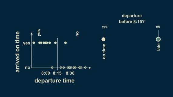
Imagine you record the time you leave home every morning and whether you arrive at work on time. Plotted, the data shows a clear pattern: leaving before about 8:15 usually means arriving on time, leaving later usually means being late.
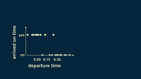
This pattern can be written as a decision tree with a single question: “Departure before 8:15?” A yes leads to the prediction “on time”, a no to “late”. The question draws a decision boundary at 8:15 and splits the data into two groups. A tree with one split like this is called a decision stump.
The rule is not perfect: there are exceptions on both sides. We can refine it by splitting each branch again. Adding boundaries at 8:00 and 8:30 gives four groups: leaving before 8:00 means on time, between 8:00 and 8:15 probably on time, between 8:15 and 8:30 probably late, and after 8:30 definitely late.
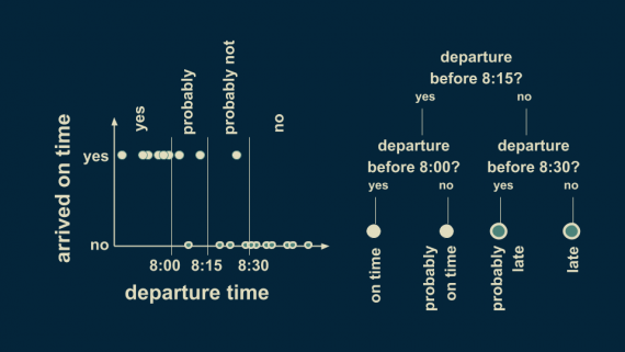
This tree has two levels. In general a tree can have as many levels as the data supports, and most implementations use binary splits, with exactly two branches per node. Here there is one input feature, departure time, and a categorical target with two values, on time or late. A tree that predicts a category is a classification tree.
Trees With Several Features
Now add a second feature: the day of the week, numbered from Monday (1) to Sunday (7). The data shows that on Saturdays and Sundays the on-time points shift to the left: leaving at 8:10 is early enough on a weekday, but not at the weekend.
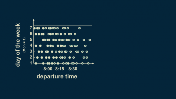
The tree starts as before, with the split at 8:15: leaving later still means being late. But leaving earlier no longer guarantees arriving on time, so the left branch is split again by a second feature: is it a weekday? On weekdays, leaving before 8:15 means arriving on time; at weekends it usually does, but not always.
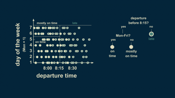
One more split, at 8:00 for weekend departures, finishes the job. The tree now divides the two-dimensional feature space into four rectangles, two for “on time” and two for “late”. It has three levels, and its branches do not all have the same depth: a tree only splits where the data needs it.
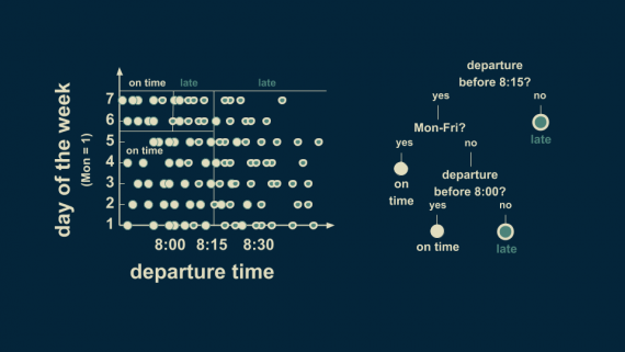
This is the geometry of every decision tree: each split is a line perpendicular to one feature axis, so the tree carves the feature space into axis-aligned boxes, and every box gets one prediction. With ten features the boxes are ten-dimensional, but the principle is the same.
Regression Trees
When the target is a continuous number, the same procedure gives a regression tree. Suppose we want to predict the time people wake up from their age. Without knowing a person’s age, the best single guess is the average of the whole dataset, about 6:25. That average is the root of the tree.
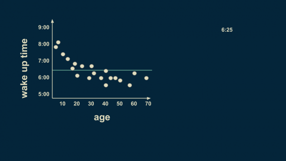
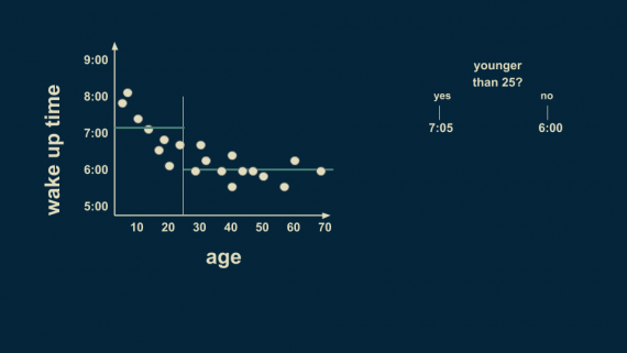
A good first split is at age 25: on average, people younger than 25 wake up at 7:05, and older people at 6:00. Each leaf predicts the mean of the training examples that fall into it.
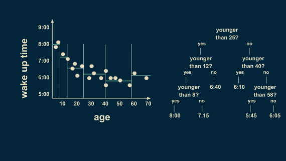
Splitting further at 12, 40, 8 and 58 gives an increasingly detailed step function. To predict the wake-up time of a 36-year-old, start at the root: younger than 25? No, go right. Younger than 40? Yes, go left. The leaf says 6:10.
A regression tree also works with several features. Add the month of the year: in this made-up dataset, children and teenagers wake up with the sun, so their wake-up time depends strongly on the season, while adults keep a more stable schedule and older people wake up slightly earlier.
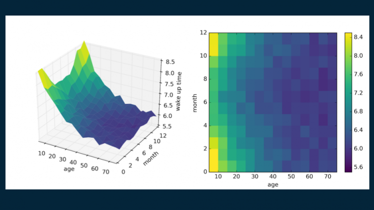
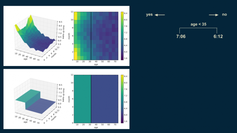
The tree starts with the overall mean, about 6:30, and then splits at age 35: younger people wake up at 7:06 on average, older ones at 6:12.
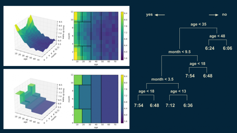
Subsequent splits separate winter from summer months for the younger group, split the older group at 48, and split the young winter group at 18 and the young summer group at 13. With every split the model, shown at the bottom left of each picture, looks more like the data at the top.
How a Tree Chooses Its Splits
In the examples above the splits were chosen by eye. A learning algorithm does it by trying every candidate split — every feature and every threshold between neighbouring values — and keeping the one that separates the data best. Then it repeats the process in each child node. This is recursive binary splitting: greedy, top-down, one node at a time. It does not guarantee the best possible tree, which is computationally intractable to find, but it works very well in practice.
“Separates best” means that the child nodes are as pure as possible: ideally each contains examples of only one class. Two measures of impurity are common.
Gini impurity
Gini = 1 − Σ pₖ²
where pₖ is the fraction of examples of class k in the node. It is the probability of mislabeling a random example if you labeled it randomly according to the class proportions in the node. A pure node has Gini 0; a 50/50 node with two classes has 0.5. Gini impurity is the default in CART and scikit-learn. It is often called the Gini index, although it is not the same as the Gini coefficient used in economics.
Entropy and information gain
Entropy = −Σ pₖ · log₂ pₖ
Entropy measures uncertainty in bits: 0 for a pure node, 1 for a 50/50 split between two classes. The information gain of a split is the entropy of the parent minus the weighted average entropy of the children. The tree picks the split with the largest gain.
A worked example
Take a node with 10 commutes: 6 on time and 4 late. The split “departure before 8:15?” sends 6 commutes left (5 on time, 1 late) and 4 right (1 on time, 3 late):
| Measure | Parent (6 / 4) | Left (5 / 1) | Right (1 / 3) | Weighted children | Gain |
|---|---|---|---|---|---|
| Gini impurity | 0.480 | 0.278 | 0.375 | 0.6 × 0.278 + 0.4 × 0.375 = 0.317 | 0.163 |
| Entropy | 0.971 | 0.650 | 0.811 | 0.6 × 0.650 + 0.4 × 0.811 = 0.715 | 0.256 |
The algorithm computes the same numbers for every other candidate split and keeps the one with the highest gain. Gini and entropy almost always choose the same splits; Gini is slightly faster because it does not need a logarithm.
Splits for regression
For a regression tree, impurity is the variance of the target in the node, equivalent to the mean squared error of predicting the node mean. The best split is the one that reduces the weighted variance of the children the most. Each leaf predicts the mean of its training examples; with mean absolute error as the criterion, it predicts the median instead.
ID3, C4.5 and CART
Several classic algorithms differ mainly in the split criterion and the shape of the tree:
| Algorithm | Author, year | Split criterion | Splits | Features and targets |
|---|---|---|---|---|
| ID3 | Ross Quinlan, 1986 | Information gain | One branch per category | Categorical features, classification only |
| C4.5 | Ross Quinlan, 1993 | Gain ratio (information gain normalized by split size) | Multiway for categories, binary for numbers | Numerical and categorical features, missing values, pruning |
| CART | Breiman, Friedman, Olshen and Stone, 1984 | Gini impurity; variance for regression | Always binary | Classification and regression, cost-complexity pruning |
scikit-learn implements an optimized version of CART, so its trees are always binary, and categorical features must be encoded as numbers. Information gain on its own favours features with many distinct values, such as IDs; the gain ratio of C4.5 corrects this.
Overfitting and Pruning
The biggest weakness of decision trees is overfitting. Go back to the wake-up time example and keep splitting the age axis until every leaf contains only one or two people. Such a tree describes the training data very well — too well. It captures not only the underlying trend, the smooth curve the data follows, but also the noise: random deviations specific to this sample. On new people its predictions are worse, not better.
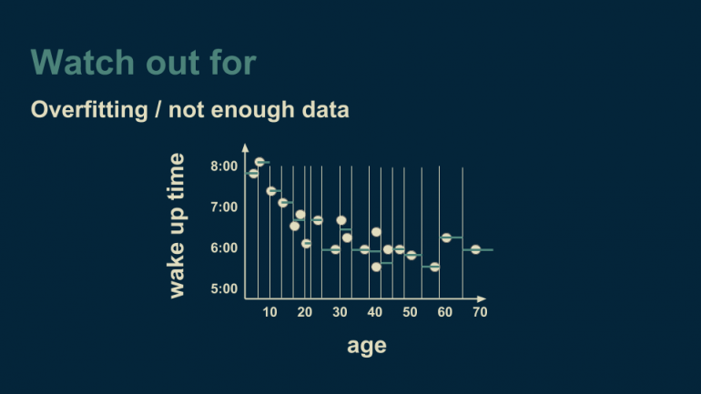
An unrestricted tree always reaches 100% training accuracy if no two identical inputs have different labels, so training accuracy says nothing about its quality. There are two ways to stop it from growing too far.
Pre-pruning, or early stopping, limits growth with hyperparameters:
max_depth— the maximum number of levels;min_samples_leaf— the minimum number of examples in a leaf, which forces each prediction to average out noise over several examples;min_samples_split— the minimum number of examples a node needs to be split;max_leaf_nodes— the maximum number of leaves;min_impurity_decrease— the minimum gain a split must achieve.
Post-pruning grows the full tree and then removes branches that do not pay for their complexity. CART uses cost-complexity pruning: it minimizes the training error plus α times the number of leaves. A larger α gives a smaller tree, and the best α is chosen by cross-validation. In scikit-learn it is the ccp_alpha parameter.
The effect of depth is easy to measure. On noisy samples of a sine wave (noise with a standard deviation of 0.3, so an RMSE of 0.3 is the best achievable), a regression tree behaves like this:
| max_depth | Leaves | Train RMSE | Test RMSE |
|---|---|---|---|
| 1 | 2 | 0.666 | 0.666 |
| 3 | 8 | 0.353 | 0.383 |
| 5 | 31 | 0.252 | 0.328 |
| Unlimited | 300 | 0.000 | 0.399 |
A stump underfits, depth 5 gets close to the noise level, and the unlimited tree has one leaf per training point: zero training error and a worse test error than depth 3.
Many features
The method itself does not care how many features there are: you can add latitude, physical activity, body mass index or anything else that might matter. Geoffrey Hinton has a famous piece of advice for picturing such spaces: imagine three dimensions and tell yourself, very loudly, that there are fourteen.
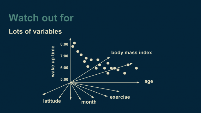
Many features do create problems. Every split has to compare more candidates, which costs computation, and the more features there are, the more data you need to choose between them reliably. When the number of examples is comparable to the number of features, a tree easily finds splits that look good by chance. Random forests counter this by considering a random subset of features at every split.
Decision Trees in Python With scikit-learn
Training a classifier
The breast cancer dataset that ships with scikit-learn has 569 tumours described by 30 numerical features, labeled malignant (0) or benign (1). Here is an unrestricted tree compared with a tree limited to three levels:
from sklearn.datasets import load_breast_cancer
from sklearn.model_selection import train_test_split
from sklearn.tree import DecisionTreeClassifier, export_text

data = load_breast_cancer()
X_train, X_test, y_train, y_test = train_test_split(
    data.data, data.target, test_size=0.25, stratify=data.target, random_state=42)

for depth in [None, 3]:
    tree = DecisionTreeClassifier(max_depth=depth, random_state=42).fit(X_train, y_train)
    print(f"max_depth={depth}: depth {tree.get_depth()}, {tree.get_n_leaves()} leaves, "
          f"train {tree.score(X_train, y_train):.3f}, test {tree.score(X_test, y_test):.3f}")

small = DecisionTreeClassifier(max_depth=2, random_state=42).fit(X_train, y_train)
print(export_text(small, feature_names=list(data.feature_names)))
Output:
max_depth=None: depth 7, 18 leaves, train 1.000, test 0.923
max_depth=3: depth 3, 7 leaves, train 0.977, test 0.944
|--- worst radius <= 16.80
|   |--- worst concave points <= 0.14
|   |   |--- class: 1
|   |--- worst concave points >  0.14
|   |   |--- class: 0
|--- worst radius >  16.80
|   |--- texture error <= 0.47
|   |   |--- class: 1
|   |--- texture error >  0.47
|   |   |--- class: 0
The unrestricted tree is perfect on the training data and worse on the test set than the tree with three levels — overfitting in action. export_text prints the learned rules, which is what makes trees so easy to explain: a tumour with a large worst radius and high texture error is classified as malignant. For a graphical version, use sklearn.tree.plot_tree with matplotlib.
Pruning, feature importance and a random forest
Instead of guessing the depth, you can compute the cost-complexity pruning path and choose ccp_alpha by cross-validation:
from sklearn.datasets import load_breast_cancer
from sklearn.model_selection import train_test_split, GridSearchCV
from sklearn.tree import DecisionTreeClassifier
from sklearn.ensemble import RandomForestClassifier

data = load_breast_cancer()
X_train, X_test, y_train, y_test = train_test_split(
    data.data, data.target, test_size=0.25, stratify=data.target, random_state=42)

# Candidate alphas from the cost-complexity pruning path of the full tree
path = DecisionTreeClassifier(random_state=42).cost_complexity_pruning_path(X_train, y_train)
search = GridSearchCV(DecisionTreeClassifier(random_state=42),
                      {"ccp_alpha": path.ccp_alphas}, cv=5)
search.fit(X_train, y_train)
best = search.best_estimator_
print(f"best ccp_alpha = {search.best_params_['ccp_alpha']:.4f}: "
      f"{best.get_n_leaves()} leaves, test accuracy {best.score(X_test, y_test):.3f}")

forest = RandomForestClassifier(n_estimators=300, random_state=42).fit(X_train, y_train)
print(f"random forest: test accuracy {forest.score(X_test, y_test):.3f}")

top = sorted(zip(best.feature_importances_, data.feature_names), reverse=True)[:3]
for importance, name in top:
    print(f"{name:>22}: {importance:.3f}")
Output:
best ccp_alpha = 0.0031: 11 leaves, test accuracy 0.937
random forest: test accuracy 0.958
          worst radius: 0.722
  worst concave points: 0.121
         texture error: 0.048
The pruned tree is smaller and more accurate than the unrestricted one. On a test set of 143 tumours, the difference between 0.937 and 0.944 is a single example, so the pruned tree and the depth-3 tree are equally good. The random forest of 300 trees beats every single tree, at the cost of interpretability. Feature importance shows how much each feature reduced impurity across all the splits of the tree: here one feature, worst radius, does most of the work.
Regression tree
The code behind the depth table in the section on overfitting:
import numpy as np
from sklearn.tree import DecisionTreeRegressor

rng = np.random.default_rng(0)
X = np.sort(rng.uniform(0, 10, 300)).reshape(-1, 1)
y = np.sin(X).ravel() + rng.normal(0, 0.3, 300)
X_test = np.linspace(0, 10, 1000).reshape(-1, 1)
y_test = np.sin(X_test).ravel() + rng.normal(0, 0.3, 1000)

for depth in [1, 3, 5, None]:
    tree = DecisionTreeRegressor(max_depth=depth, random_state=0).fit(X, y)
    rmse = lambda X_, y_: np.sqrt(np.mean((tree.predict(X_) - y_) ** 2))
    print(f"max_depth={str(depth):>4}: {tree.get_n_leaves():>3} leaves, "
          f"train RMSE {rmse(X, y):.3f}, test RMSE {rmse(X_test, y_test):.3f}")
Output:
max_depth=   1:   2 leaves, train RMSE 0.666, test RMSE 0.666
max_depth=   3:   8 leaves, train RMSE 0.353, test RMSE 0.383
max_depth=   5:  31 leaves, train RMSE 0.252, test RMSE 0.328
max_depth=None: 300 leaves, train RMSE 0.000, test RMSE 0.399
Advantages and Disadvantages
| Advantages | Disadvantages |
|---|---|
| Easy to read, draw and explain; predictions can be traced as rules | Overfits easily without depth limits or pruning |
| No feature scaling or normalization needed | Unstable: a small change in the data can produce a very different tree |
| Handles numerical and categorical features; scikit-learn also supports missing values natively | Axis-aligned splits approximate diagonal boundaries with many small steps |
| Captures nonlinear relationships and feature interactions automatically | Predictions are piecewise constant; a regression tree cannot extrapolate beyond the training range |
| Fast to train and to predict | Usually less accurate than random forests or gradient boosting |
| Can detect abrupt jumps and spikes that smooth models such as linear regression miss | Greedy splitting does not find the globally optimal tree |
Decision trees are a good choice when you want to make few assumptions about your data and need a model you can explain: credit scoring rules, medical triage, customer segmentation, or a first baseline on a new tabular dataset.
Decision Tree vs Random Forest vs Gradient Boosting
The instability of single trees turns into a strength when many trees are combined:
- A random forest trains hundreds of deep trees, each on a bootstrap sample of the data and with a random subset of features at every split, and averages them. Averaging cancels out much of the variance of the individual trees, so the forest is far more accurate and robust than one tree and still needs little tuning.
- Gradient boosting trains shallow trees one after another, each correcting the errors of the ensemble so far. Implementations such as XGBoost, LightGBM and CatBoost are usually the most accurate models for tabular data.
Both give up the readability of a single tree. A common workflow is to start with a single shallow tree to understand the data, then move to an ensemble for accuracy and use feature importance or SHAP values to explain it.
FAQ
What is a decision tree in machine learning?
It is a supervised learning model that predicts a target by applying a sequence of if-then rules learned from data. Each internal node tests one feature, each branch is an outcome of the test, and each leaf gives a prediction.
What is the difference between a classification tree and a regression tree?
A classification tree predicts a category and chooses splits by Gini impurity or entropy; each leaf predicts the most common class. A regression tree predicts a number and chooses splits by variance reduction; each leaf predicts the average of its training examples.
What is the difference between Gini impurity and entropy?
Both measure how mixed the classes in a node are and are zero for a pure node. Entropy comes from information theory and uses logarithms; Gini is slightly cheaper to compute. In practice they lead to nearly identical trees.
How do you prevent a decision tree from overfitting?
Limit its growth with max_depth, min_samples_leaf or max_leaf_nodes, or grow it fully and prune it with cost-complexity pruning, choosing the parameters by cross-validation. Or use an ensemble such as a random forest.
Is a decision tree better than a random forest?
A single tree is easier to interpret and faster, but a random forest is almost always more accurate and less sensitive to the particular training sample. Use a tree when you need to explain the rules, a forest when you need accuracy.
See also: our guide to gradient boosting, which builds the most accurate tabular models from shallow decision trees, and a list of websites with public datasets to practice decision trees on.