Backpropagation Explained: Algorithm, Example and Python Code

Backpropagation (backward propagation of errors) is the algorithm that computes how much each weight in a neural network contributed to the error, so that gradient descent can adjust it. It applies the chain rule of calculus layer by layer, starting at the loss and moving back toward the input, and reuses intermediate results so that the gradient for every weight costs roughly as much as one extra forward pass. Every modern network, from small classifiers to large language models, is trained this way.

This guide explains backpropagation step by step: the forward pass, the chain rule, the three equations that make up the algorithm, a worked numerical example, the matrix form used in practice, a NumPy implementation with a gradient check, how PyTorch autograd does the same thing, and why gradients vanish or explode in deep networks.

What Is Backpropagation?

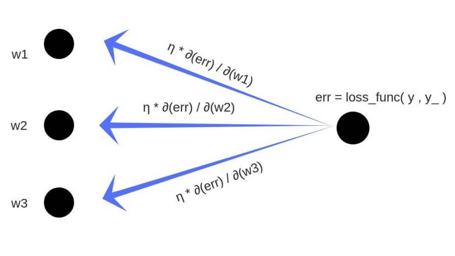
A neural network makes a prediction, a loss function measures how wrong it is, and training has to decide how to change millions of weights to make the loss smaller. For that it needs the gradient: the partial derivative of the loss with respect to each weight, which says in which direction and how strongly that weight pushes the error up or down.

Backpropagation is the efficient way to get all of those derivatives at once. The idea is simple: adjust each weight in proportion to how much it contributes to the overall error. The error is computed at the output; backpropagation then sends it back through the network, and at every layer works out the share of the error that belongs to each weight.

It is easy to confuse backpropagation with gradient descent. Backpropagation computes the gradients; gradient descent uses them to update the weights. Together they form one training step.

The method has a long history. Seppo Linnainmaa described reverse-mode automatic differentiation, the general algorithm behind it, in 1970; Paul Werbos proposed applying it to neural networks in 1974; and the 1986 paper by David Rumelhart, Geoffrey Hinton and Ronald Williams showed that it trains multilayer networks to learn useful internal representations, which made it the standard training method.

The Forward Pass

Backpropagation always follows a forward pass (forward propagation), in which the input flows through the network to produce a prediction and the loss. Take the smallest interesting network: an input X, one hidden neuron and one output neuron, with weights Wh and Wo:

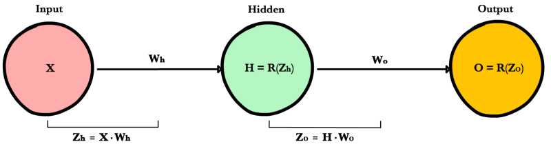
Each neuron first computes a weighted input Z, then applies an activation function R, here ReLU. The loss is the squared error between the prediction ŷ and the target y. These three building blocks and their derivatives are all backpropagation needs:

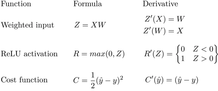
Written out, the forward pass is Zh = X·Wh, H = R(Zh), Zo = H·Wo, ŷ = O = R(Zo), and the loss is C = ½(ŷ − y)². During this pass the network stores the intermediate values Z and H — the backward pass will need them.

The Chain Rule

A network is a chain of nested functions: each layer takes the output of the previous one. With three functions g, h and k the forward pass is

f(x) = g(h(k(x)))

The chain rule says that the derivative of a composition is the product of the derivatives of its parts, each taken at the point where that function is evaluated:

f′(x) = g′(h(k(x))) · h′(k(x)) · k′(x)

It is easier to read with names for the intermediate values. Let u = k(x) and v = h(u), so that f = g(v). Then

df/dx = df/dv · dv/du · du/dx = g′(v) · h′(u) · k′(x)

The same rule gives the derivative with respect to any intermediate value: just stop multiplying when you reach it. For example, df/du = g′(v) · h′(u). This is exactly what backpropagation does. In a network the intermediate values are the weighted inputs Z and activations H of each layer, the outermost function is the loss C, and the derivatives of the loss with respect to the intermediate values are the layer errors used below.

Deriving the Gradients

For a single neuron with weight W, the loss is C(R(Z(XW))), and the chain rule gives

∂C/∂W = C′(R) · R′(Z) · Z′(W) = (ŷ − y) · R′(Z) · X

For the two-layer network above, the derivative with respect to the output weight Wo is

∂C/∂Wo = (ŷ − y) · R′(Zo) · H

and for the hidden weight Wh we keep applying the chain rule until we reach the function that contains Wh:

∂C/∂Wh = (ŷ − y) · R′(Zo) · Wo · R′(Zh) · X

Notice the pattern. Each layer deeper adds two factors — a weight and an activation derivative — to factors that were already computed for the layers above it. In a network with four layers the expressions look like this:

Computing every expression from scratch would repeat the same multiplications over and over, and the work would grow quadratically with depth. Backpropagation avoids this with memoization: it computes each shared factor once, stores it, and passes it back to the previous layer.

The Three Equations of Backpropagation

The stored factor is called the layer error: the derivative of the loss with respect to the weighted input Z of a layer. It answers the question: how does the loss change if the input to this layer changes? Three equations then cover everything.

1. Output layer error

Eo = (ŷ − y) · R′(Zo)

The derivative of the loss with respect to the prediction, times the derivative of the output activation.

2. Hidden layer error

Eh = Eo · Wo · R′(Zh)

The error of the next layer, sent back through the weights that connect the two layers and multiplied by the derivative of this layer’s activation. This is the heart of backpropagation: each layer receives the weighted error of the layer after it, and the process repeats until it reaches the first hidden layer.

3. Gradient for any weight

∂C/∂W = error of the layer · input of the layer

For the two weights in our network this gives ∂C/∂Wo = Eo · H and ∂C/∂Wh = Eh · X. The input of a layer is the activation of the previous layer, not its weighted input Z.

These three equations replace all the long chain-rule expressions. The cost of the backward pass is now proportional to the size of the network, about the same as the forward pass — in practice the backward pass takes roughly twice as long as the forward one, because it computes gradients for both the weights and the activations.

Worked Example With Numbers

Let us run one full training step on the network above with concrete numbers: input X = 1.5, target y = 1, initial weights Wh = 0.8 and Wo = 2.0, learning rate 0.1.

Step	Computation	Value
Forward	Zh = X · Wh = 1.5 × 0.8	1.20
Forward	H = ReLU(Zh)	1.20
Forward	Zo = H · Wo = 1.2 × 2.0	2.40
Forward	ŷ = ReLU(Zo)	2.40
Loss	C = ½ (2.4 − 1)²	0.980
Backward	Eo = (ŷ − y) · R′(Zo) = 1.4 × 1	1.40
Backward	∂C/∂Wo = Eo · H = 1.4 × 1.2	1.68
Backward	Eh = Eo · Wo · R′(Zh) = 1.4 × 2.0 × 1	2.80
Backward	∂C/∂Wh = Eh · X = 2.8 × 1.5	4.20
Update	Wo = 2.0 − 0.1 × 1.68	1.832
Update	Wh = 0.8 − 0.1 × 4.20	0.380
Check	Loss with the new weights	0.001

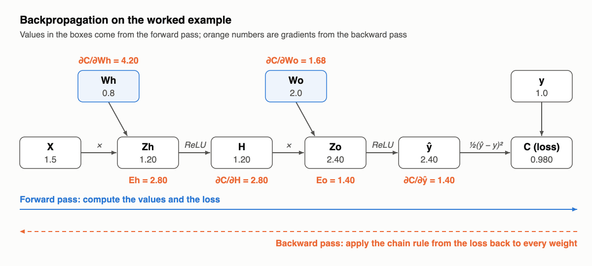
One step brings the loss from 0.98 to 0.001. You can confirm the gradients numerically: nudging Wo by a tiny amount ε and measuring (C(Wo + ε) − C(Wo − ε)) / 2ε gives 1.68 for Wo and 4.20 for Wh, exactly what backpropagation produced.

Backpropagation in Matrix Form

Real layers have many neurons, and real training processes a batch of examples at once, so the same three equations are written with matrices. For layer l with weights W(l), bias b(l), weighted input Z(l) = A(l−1)W(l) + b(l) and activation A(l) = σ(Z(l)):

Equation	Matrix form	Meaning
Output error	δ(L) = ∂C/∂A(L) ⊙ σ′(Z(L))	Loss gradient times activation derivative, element-wise
Hidden error	δ(l) = (δ(l+1) W(l+1)T) ⊙ σ′(Z(l))	Error sent back through the transposed weights
Weight gradient	∂C/∂W(l) = A(l−1)T δ(l)	Layer input times layer error, summed over the batch
Bias gradient	∂C/∂b(l) = Σ δ(l)	Layer error summed over the batch

Here ⊙ is element-wise multiplication. Rows are examples and columns are neurons, the convention used by NumPy and PyTorch. Two common combinations simplify the output error: with a sigmoid output and binary cross-entropy loss, or a softmax output and cross-entropy loss, δ(L) is simply ŷ − y, the prediction minus the label.

The Training Algorithm, Step by Step

1. Initialize the weights with small random values (for example, He or Xavier initialization) and the biases with zeros.
2. Forward pass: feed a mini-batch through the network, storing every Z and A.
3. Compute the loss between predictions and targets.
4. Backward pass: compute the output error, then move layer by layer toward the input, computing each layer error and the gradients of its weights and biases.
5. Update every weight with gradient descent or an optimizer such as Adam: W ← W − η · ∂C/∂W.
6. Repeat for the next mini-batch until the validation loss stops improving.

Why updates for different examples do not cancel out

The worked example above uses a single training point, but a network is not trained to fit one point after another. Training minimizes the average loss over the whole training set, L(W) = (1/n) · Σ Lᵢ(W). Its gradient is the average of the per-example gradients, and this is what backpropagation computes for a batch: in the NumPy code below, the division by n in dZ2 = (P - y) / n does exactly that.

Per-example gradients often disagree. At the start of training our two moons network, 253 of the 1,000 examples have a gradient that points against the full-batch gradient: a step that helps the training set as a whole makes the loss on those examples slightly worse. Averaging resolves the conflict. Examples that pull the weights in opposite directions partly cancel each other, the direction on which most examples agree wins, and with a small enough learning rate the total loss goes down at every step.

With stochastic or mini-batch gradient descent each step sees only part of the data, so a single step can increase the total loss. On average, though, the gradient of a random mini-batch equals the full gradient, so the noise evens out over many steps, and a decreasing learning rate lets the weights settle. Trained one example at a time (batch size 1, learning rate 0.1), the same network reaches about 95% accuracy after 5 epochs.

The weights can get stuck in a compromise that is equally wrong for every example, but that is a question of model capacity, not of backpropagation. A model without a hidden layer cannot represent XOR, and the best it can do is to predict 0.5 for all four points. Add a hidden layer with four neurons, and the same training procedure gets all four points right. The networks used in practice have more than enough capacity to fit their training data; the real risk is the opposite, overfitting, which is controlled with validation data and regularization.

Backpropagation From Scratch in Python

The code below trains a network with two inputs, 16 hidden neurons with tanh and a sigmoid output on the two moons dataset from scikit-learn. The backward function is a direct translation of the matrix equations above:

import numpy as np
from sklearn.datasets import make_moons

X, y = make_moons(n_samples=1000, noise=0.2, random_state=0)
y = y.reshape(-1, 1)
rng = np.random.default_rng(0)

# 2 inputs -> 16 hidden (tanh) -> 1 output (sigmoid)
W1 = rng.normal(0, 1, (2, 16)) * np.sqrt(1 / 2)
b1 = np.zeros((1, 16))
W2 = rng.normal(0, 1, (16, 1)) * np.sqrt(1 / 16)
b2 = np.zeros((1, 1))

def sigmoid(z):
    return 1 / (1 + np.exp(-z))

def forward(X):
    Z1 = X @ W1 + b1
    A1 = np.tanh(Z1)
    Z2 = A1 @ W2 + b2
    P = sigmoid(Z2)
    return Z1, A1, Z2, P

def loss(P, y):                                  # binary cross-entropy
    return -np.mean(y * np.log(P + 1e-12) + (1 - y) * np.log(1 - P + 1e-12))

def backward(X, y, A1, P):
    n = len(X)
    dZ2 = (P - y) / n                            # error of the output layer
    dW2 = A1.T @ dZ2                             # error x input of the layer
    db2 = dZ2.sum(axis=0, keepdims=True)
    dZ1 = (dZ2 @ W2.T) * (1 - A1 ** 2)           # send error back, times tanh'
    dW1 = X.T @ dZ1
    db1 = dZ1.sum(axis=0, keepdims=True)
    return dW1, db1, dW2, db2

lr = 1.0
for epoch in range(2001):
    Z1, A1, Z2, P = forward(X)
    dW1, db1, dW2, db2 = backward(X, y, A1, P)
    W1 -= lr * dW1; b1 -= lr * db1               # gradient descent step
    W2 -= lr * dW2; b2 -= lr * db2
    if epoch % 500 == 0:
        acc = np.mean((P > 0.5) == y)
        print(f"epoch {epoch:4d}: loss = {loss(P, y):.4f}, accuracy = {acc:.3f}")

Output:

epoch    0: loss = 0.6723, accuracy = 0.517
epoch  500: loss = 0.1061, accuracy = 0.962
epoch 1000: loss = 0.0902, accuracy = 0.966
epoch 1500: loss = 0.0839, accuracy = 0.966
epoch 2000: loss = 0.0820, accuracy = 0.968

Gradient checking

Hand-written backpropagation is easy to get subtly wrong: the network may still train, just worse. The standard test is to compare the analytic gradients with numerical ones from finite differences. Run this right after defining the functions, before the training loop:

# Gradient check: compare backprop with finite differences
Z1, A1, Z2, P = forward(X)
dW1, db1, dW2, db2 = backward(X, y, A1, P)
eps = 1e-5
numeric = np.zeros_like(W1)
for i in range(W1.shape[0]):
    for j in range(W1.shape[1]):
        W1[i, j] += eps;     plus = loss(forward(X)[3], y)
        W1[i, j] -= 2 * eps; minus = loss(forward(X)[3], y)
        W1[i, j] += eps
        numeric[i, j] = (plus - minus) / (2 * eps)
rel_error = np.linalg.norm(dW1 - numeric) / np.linalg.norm(dW1 + numeric)
print(f"relative error: {rel_error:.2e}")

Output:

relative error: 5.56e-11

A relative error below about 1e-7 means the implementation is correct; values around 1e-2 or larger point to a bug. Gradient checking is far too slow for training — it needs two forward passes per weight — but it is invaluable for debugging.

Automatic Differentiation and PyTorch

Nobody writes backward passes by hand for real models. Frameworks use automatic differentiation (autodiff) in reverse mode, which is backpropagation generalized to any program. During the forward pass, PyTorch records every operation in a computational graph; each operation knows its own local derivative. Calling loss.backward() walks the graph from the loss back to the inputs, applies the chain rule at every node and stores the result in the .grad attribute of each tensor that has requires_grad=True.

Here is the same network in PyTorch, starting from the same initial weights as the NumPy version. Autograd produces the same gradients:

import torch

# Copy the initial NumPy weights (before training) into tensors that track gradients
W1_t, b1_t, W2_t, b2_t = (torch.tensor(a, requires_grad=True) for a in (W1, b1, W2, b2))
X_t, y_t = torch.tensor(X), torch.tensor(y, dtype=torch.float64)

P_t = torch.sigmoid(torch.tanh(X_t @ W1_t + b1_t) @ W2_t + b2_t)   # forward pass
loss_t = torch.nn.functional.binary_cross_entropy(P_t, y_t)
loss_t.backward()                                                   # backward pass

Z1, A1, Z2, P = forward(X)
for name, t, g in zip(["W1", "b1", "W2", "b2"], (W1_t, b1_t, W2_t, b2_t), backward(X, y, A1, P)):
    print(f"{name}: max difference = {np.abs(t.grad.numpy() - g).max():.1e}")

Output:

W1: max difference = 4.9e-17
b1: max difference = 2.4e-17
W2: max difference = 1.1e-16
b2: max difference = 0.0e+00

The differences are at the level of floating-point rounding: PyTorch’s backward() computes exactly what our hand-written function does. In a normal training loop you would call optimizer.zero_grad(), run the forward pass, call loss.backward() and then optimizer.step(); JAX and TensorFlow provide the same capability through jax.grad and tf.GradientTape.

Vanishing and Exploding Gradients

The hidden layer equation multiplies the error by a weight and an activation derivative at every layer. In a deep network these factors pile up: if they are typically smaller than 1, the gradient shrinks exponentially on its way to the first layers — the vanishing gradient problem. If they are larger than 1, it grows exponentially — exploding gradients. The early layers then either stop learning or receive huge, destabilizing updates.

The sigmoid is a classic cause: its derivative is at most 0.25, so every sigmoid layer cuts the gradient by at least a factor of four. The experiment below measures the gradient that reaches the first and the last layer of a 20-layer network:

import torch
import torch.nn as nn

def gradient_norms(activation, he_init=False, depth=20, width=64):
    torch.manual_seed(0)
    layers = []
    for _ in range(depth):
        linear = nn.Linear(width, width)
        if he_init:
            nn.init.kaiming_normal_(linear.weight, nonlinearity="relu")
            nn.init.zeros_(linear.bias)
        layers += [linear, activation()]
    model = nn.Sequential(*layers, nn.Linear(width, 1))
    loss = model(torch.randn(256, width)).pow(2).mean()
    loss.backward()
    return model[0].weight.grad.norm().item(), model[-1].weight.grad.norm().item()

for label, act, he in [("sigmoid", nn.Sigmoid, False),
                       ("ReLU, default init", nn.ReLU, False),
                       ("ReLU, He init", nn.ReLU, True)]:
    first, last = gradient_norms(act, he)
    print(f"{label:>18}: first layer {first:.1e}, last layer {last:.1e}")

Output:

           sigmoid: first layer 7.1e-19, last layer 5.8e-01
ReLU, default init: first layer 3.3e-10, last layer 9.2e-03
     ReLU, He init: first layer 5.7e-02, last layer 7.3e-01

With sigmoid, the gradient at the first layer is 18 orders of magnitude smaller than at the last: those layers effectively do not learn. ReLU helps, but only together with initialization scaled for it. The standard remedies are:

• ReLU-family activations (ReLU, GELU, SiLU), whose derivative does not saturate for positive inputs.
• Proper initialization: He initialization for ReLU, Xavier (Glorot) for tanh, so that the signal keeps the same scale from layer to layer.
• Normalization layers: batch normalization in CNNs, layer normalization in Transformers.
• Residual connections: the skip connections of ResNet and Transformers give the gradient a direct path to earlier layers, which is what makes networks with hundreds of layers trainable.
• Gradient clipping against explosions: torch.nn.utils.clip_grad_norm_ rescales the gradients when their norm exceeds a threshold.

Backpropagation Through Time

Recurrent neural networks apply the same weights at every time step. To train them, the network is unrolled over the sequence into one long feedforward graph, and ordinary backpropagation is run through it. This is called backpropagation through time (BPTT). Because the same weights are multiplied again at every step, RNNs suffer badly from vanishing and exploding gradients over long sequences; LSTM and GRU cells were designed to fix this, and Transformers avoid the problem by processing the whole sequence in parallel with attention. For long sequences, truncated BPTT backpropagates only through the last few dozen or hundred steps.

FAQ

What is backpropagation in simple terms?

It is the way a neural network finds out which weights are responsible for its mistakes. The error is measured at the output and passed backward through the network, layer by layer, and each weight gets a number that says how to change it to reduce the error.

What is the difference between backpropagation and gradient descent?

Backpropagation computes the gradient of the loss with respect to every weight. Gradient descent is the optimization algorithm that uses those gradients to update the weights. You need both to train a network.

What is the difference between the forward pass and the backward pass?

The forward pass runs the input through the network to compute the prediction and the loss. The backward pass runs from the loss back to the input to compute the gradients. A training step is one forward pass, one backward pass and one weight update.

Why is it called backpropagation?

Because the error propagates backward: it is computed at the output and passed from each layer to the one before it, the opposite direction to the data in the forward pass.

Is backpropagation used in large language models?

Yes. GPT-style models, diffusion models and practically every other modern network are trained with backpropagation and an Adam-family optimizer. The scale is different, but the algorithm is the same as in the small example above.

See also: our guides to gradient descent, which uses the gradients that backpropagation computes, and to activation functions, whose derivatives appear in every backward step.