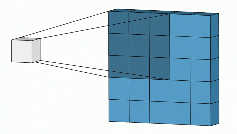
A convolutional neural network (CNN, or ConvNet) is a type of neural network designed for data with a grid structure, above all images. Instead of connecting every input pixel to every neuron, a CNN slides small learnable filters across the image and detects the same local patterns — edges, textures, shapes — wherever they appear. Stacking such layers builds a visual hierarchy, from simple edges in the first layers to whole objects in the last ones. CNNs power image classification, object detection, segmentation and medical imaging, and they remain one of the core architectures of deep learning.
This guide explains how a convolutional neural network works step by step: the convolution operation, padding and stride, channels and filters, pooling, why convolutions need so few parameters, what the filters actually learn, receptive fields, the classic CNN architectures, and how to build and train a CNN in PyTorch.
Key takeaways
- Convolution: a small matrix of weights, the kernel, slides over the image and computes a weighted sum at every position, producing a feature map.
- Two built-in assumptions make CNNs efficient: local connectivity (each output depends on a small neighbourhood) and weight sharing (the same kernel is used everywhere).
- Building blocks: convolutional layers, activation functions, pooling or strided convolutions to shrink the image, and a classifier head.
- Hierarchy: early layers detect edges, middle layers textures and parts, deep layers whole objects, because the receptive field grows with depth.
- Today CNNs such as ResNet and ConvNeXt compete with vision Transformers and are preferred when data or compute are limited.
What Is a Convolutional Neural Network?
An ordinary fully connected network treats an image as a long list of numbers: it flattens a 224×224 colour image into 150,528 inputs and connects each of them to every neuron of the next layer. This ignores the most important property of images — nearby pixels are related — and needs an enormous number of weights.
A CNN keeps the image as a grid and processes it with a few types of layers:
- Convolutional layers apply learnable filters to small regions of the input and produce feature maps that show where each pattern occurs.
- Activation functions, usually ReLU, add nonlinearity after each convolution; see our guide to activation functions.
- Pooling layers or strided convolutions reduce the spatial size, so deeper layers see larger parts of the image.
- A classifier head, typically global average pooling followed by a fully connected layer, turns the final feature maps into class scores.
The network is trained like any other: the filters start random and are learned with backpropagation and gradient descent. The idea goes back to Yann LeCun’s LeNet in the late 1980s, which read handwritten digits; CNNs took over computer vision in 2012, when AlexNet won the ImageNet competition with a top-5 error of 15.3% against 26.2% for the runner-up.
How 2D Convolution Works
The core operation is surprisingly simple. Start with a kernel, a small matrix of weights, for example 3×3. The kernel slides over the two-dimensional input; at each position it multiplies its weights element-wise with the input values beneath it, sums the results and writes a single output pixel. Repeating this at every position turns one 2D matrix into another: a feature map.
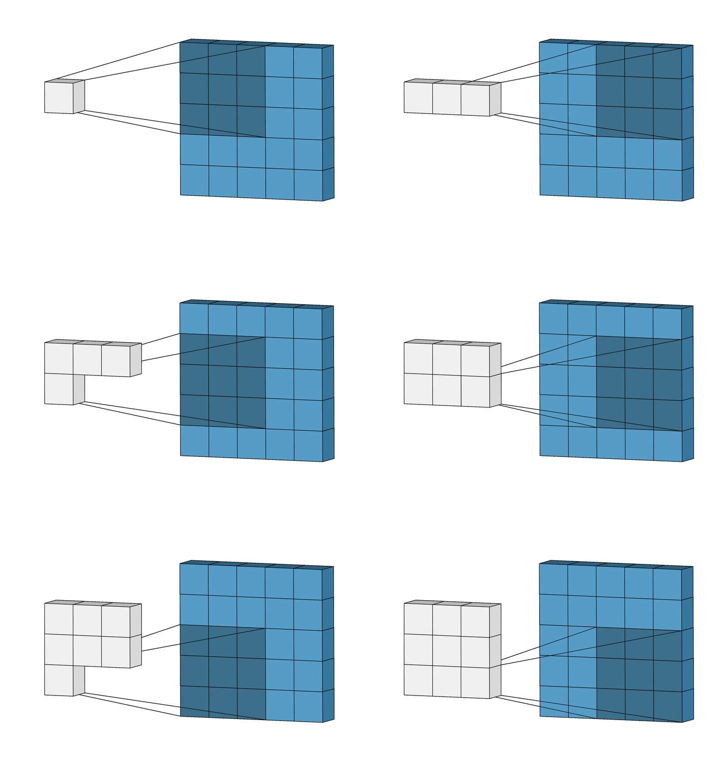
Each output value is a weighted sum of the input values located in roughly the same place as the output pixel, and the weights are the values of the kernel itself. The size of the kernel determines how many input features are combined into each output feature.
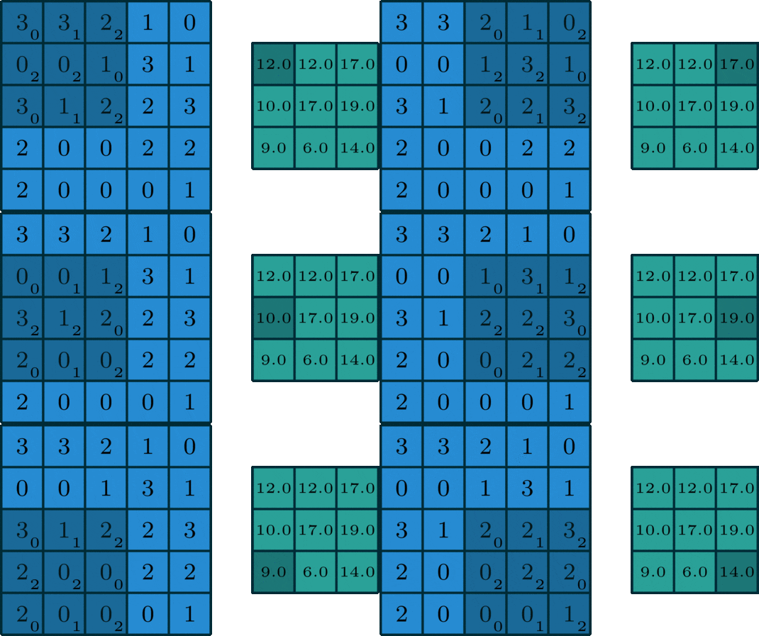
In the example above, a 5×5 input produces a 3×3 output. A fully connected layer between them would need a weight matrix of 25 × 9 = 225 parameters, with every output depending on every input. The convolution does the job with just the 9 weights of the kernel, because each output only looks at the inputs in its neighbourhood. This difference is what makes CNNs practical, and we will come back to it below.
Strictly speaking, deep learning libraries compute a cross-correlation: the kernel is not flipped as in the mathematical definition of convolution. Since the kernel weights are learned, the distinction does not matter in practice.
Padding and Stride
Padding
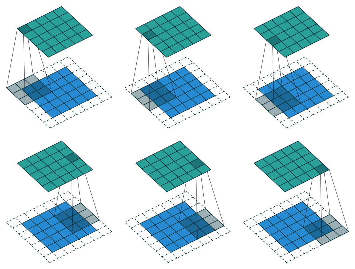
Look at the animation again: the edges get trimmed, and a 5×5 input becomes a 3×3 output. Pixels at the border never land in the centre of the kernel, because the kernel would stick out past the edge. Usually we want the output to keep the size of the input. Padding adds fake pixels around the border, normally zeros (zero padding), so the kernel can be centred on every real pixel:
Stride
Often we want the opposite: a smaller output. This is standard in CNNs, where the spatial size shrinks as the number of channels grows. One way to do it is with a pooling layer; another is the stride, the step with which the kernel moves. A stride of 1 visits every position; a stride of 2 skips every other position and roughly halves each dimension, a stride of 3 divides it by three, and so on.
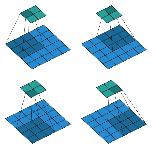
Modern architectures such as ResNet largely replace pooling in the inner layers with strided convolutions. Kernel size k, padding p and stride s determine the output size for an input of size n:
output size = ⌊(n + 2p − k) / s⌋ + 1
| Input | Kernel | Padding | Stride | Output |
|---|---|---|---|---|
| 5×5 | 3×3 | 0 | 1 | 3×3 |
| 6×6 | 3×3 | 1 (“same”) | 1 | 6×6 |
| 6×6 | 3×3 | 1 | 2 | 3×3 |
| 224×224 | 7×7 | 3 | 2 | 112×112 |
The last row is the first layer of ResNet. Here is a convolution written from scratch in NumPy, applied to a small image with a vertical edge and a Sobel kernel that detects such edges:
import numpy as np

def conv2d(image, kernel, stride=1, padding=0):
    """2D convolution (cross-correlation, as in deep learning libraries)."""
    image = np.pad(image, padding)
    k = kernel.shape[0]
    out_size = (image.shape[0] - k) // stride + 1
    out = np.zeros((out_size, out_size))
    for i in range(out_size):
        for j in range(out_size):
            patch = image[i * stride:i * stride + k, j * stride:j * stride + k]
            out[i, j] = np.sum(patch * kernel)      # multiply element-wise, then sum
    return out

# A 6x6 image: dark on the left, bright on the right
image = np.array([[0, 0, 0, 9, 9, 9]] * 6, dtype=float)
sobel_x = np.array([[-1, 0, 1],
                    [-2, 0, 2],
                    [-1, 0, 1]], dtype=float)        # detects vertical edges

print(conv2d(image, sobel_x))
print("padding=1:", conv2d(image, sobel_x, padding=1).shape)
print("stride=2: ", conv2d(image, sobel_x, stride=2, padding=1).shape)
Output:
[[ 0. 36. 36.  0.]
 [ 0. 36. 36.  0.]
 [ 0. 36. 36.  0.]
 [ 0. 36. 36.  0.]]
padding=1: (6, 6)
stride=2:  (3, 3)
The output is zero over the flat areas and large where the brightness changes: the kernel has found the edge. The result is identical to PyTorch’s torch.nn.functional.conv2d on the same input.
Channels, Filters and Kernels
So far the input had a single channel. Real images usually have three — red, green and blue — and inside the network the number of channels grows to hundreds.
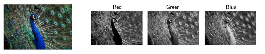
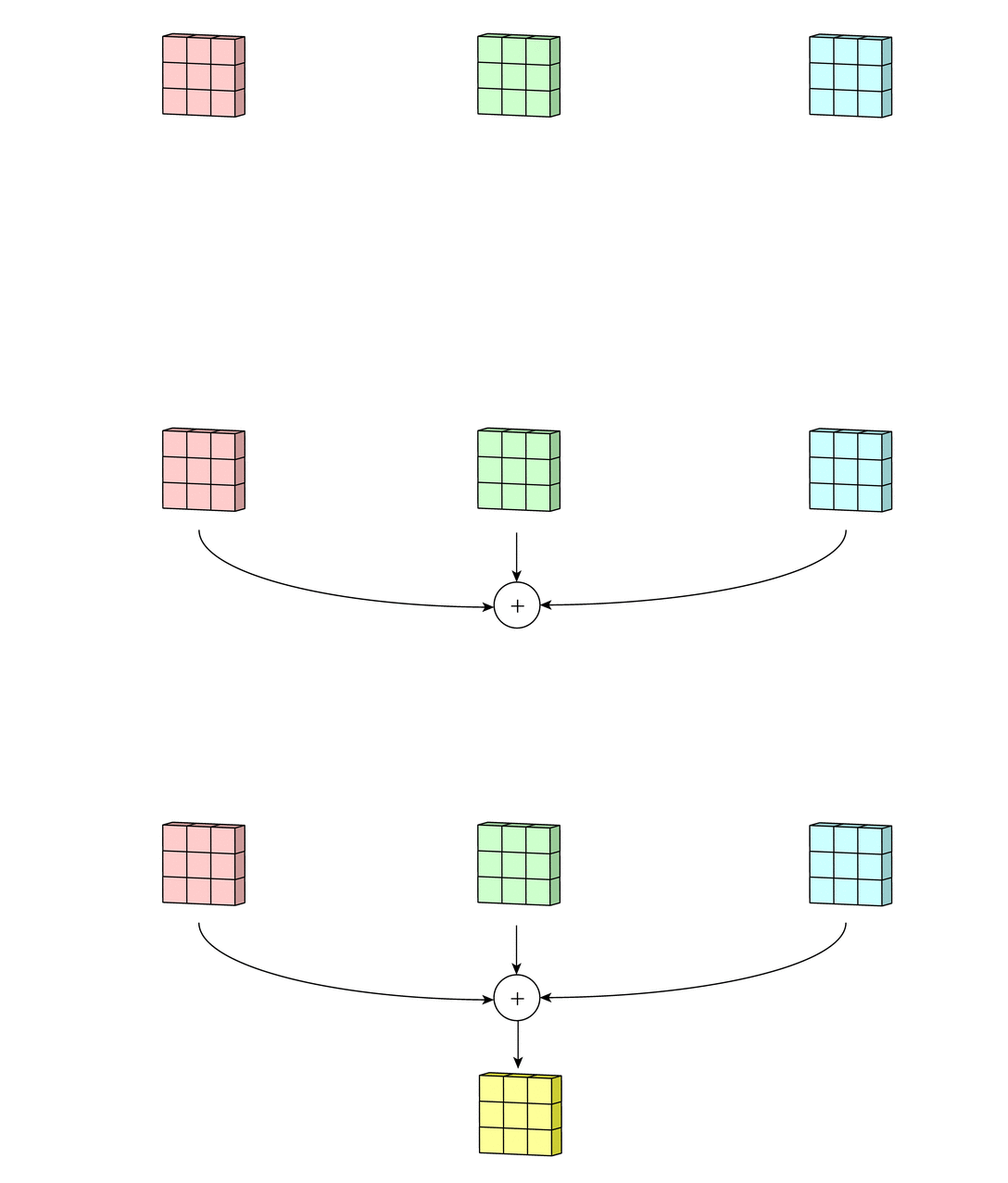
With several channels, the terms kernel and filter mean different things. A filter is a collection of kernels, one for each input channel, and each kernel is different:
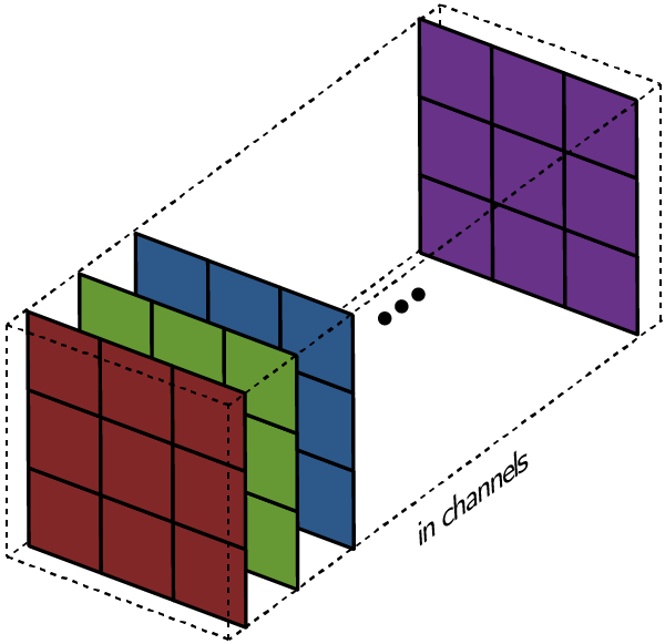
Each filter produces exactly one output channel. Every kernel of the filter slides over its own input channel and produces a processed version of it. Some kernels may get larger weights than others, so that the filter pays more attention to certain channels — for example, it can react more strongly to the red channel.
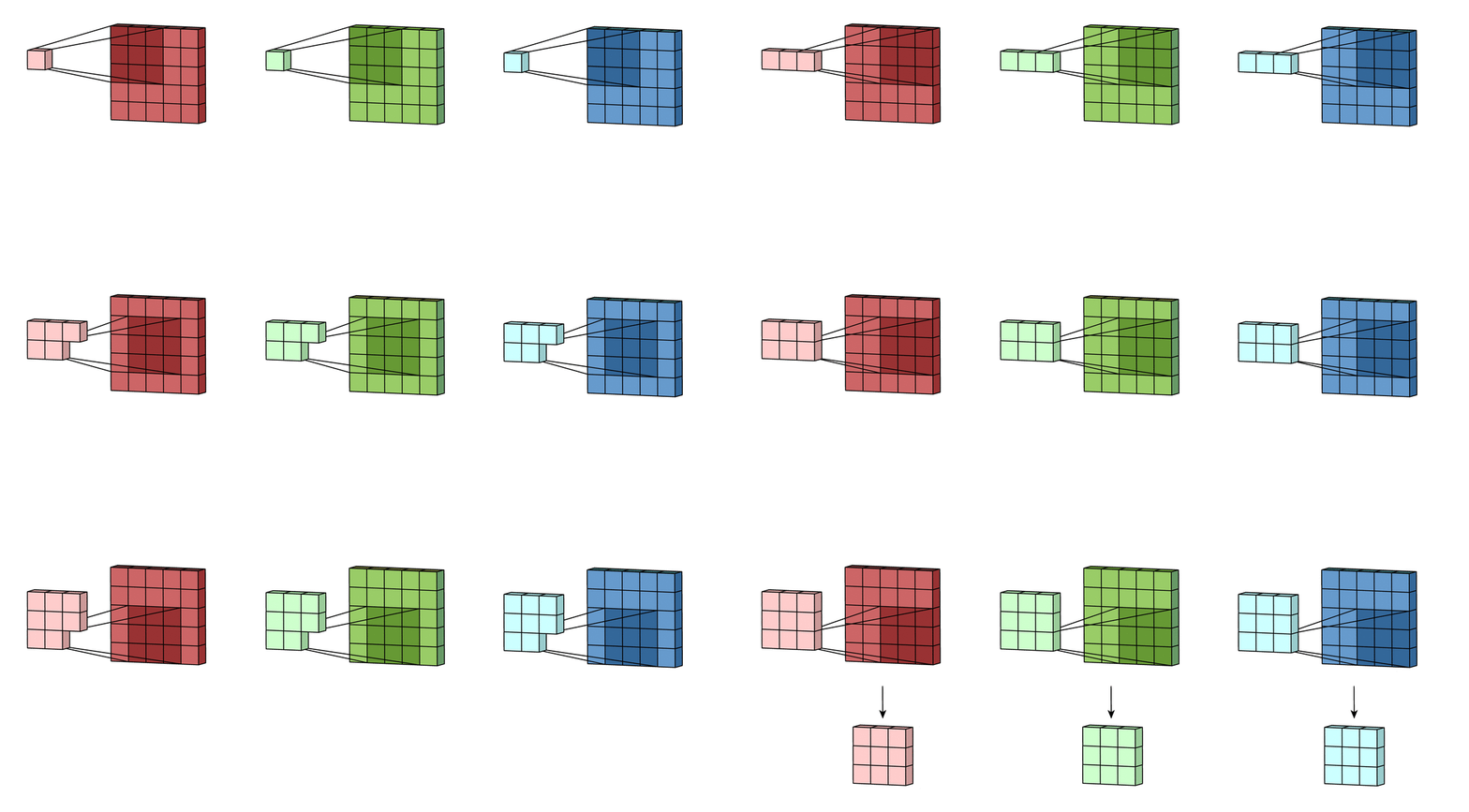
The processed versions are then summed into a single channel:
Finally, each filter has a bias, a single number added to every value of its output channel:
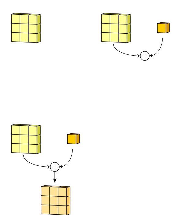
A layer with several filters repeats this for each of them and stacks the resulting channels, so the number of output channels equals the number of filters. A nonlinearity is applied, and the next convolutional layer repeats the process. The number of parameters in a convolutional layer follows directly:
parameters = (k × k × Cin + 1) × Cout
For a 3×3 convolution from 3 input channels to 64 output channels that is (3 × 3 × 3 + 1) × 64 = 1,792 parameters, regardless of whether the image is 32×32 or 4000×3000 pixels.
Pooling Layers
A pooling layer shrinks a feature map by summarizing small windows. Max pooling takes the largest value in each window, typically 2×2 with a stride of 2, which halves the width and height; average pooling takes the mean. Pooling has no parameters, makes the network slightly tolerant to small shifts of the input, and reduces the computation for the following layers.
Global average pooling averages each whole feature map into a single number. It is the standard way to end a modern CNN: a 7×7×2048 output of ResNet-50 becomes a vector of 2,048 values for the classifier, whatever the input size.
Why Convolutions Work So Well for Images
Even with all this machinery, it may not be obvious how a convolutional layer relates to an ordinary layer, or why it works so much better for images. Take a 4×4 input that we want to map to a 2×2 output. A fully connected layer would flatten the input into a vector of 16 values and multiply it by a weight matrix with 16 × 4 = 64 independent weights:

A 3×3 convolution with the same input and output is also a linear transformation, and it can be written as a matrix of the same shape. But this matrix looks very different:

Of the 64 entries, only 9 distinct parameters appear, each reused several times, and the rest are fixed at zero: every output depends only on the inputs under the kernel. A convolution is a fully connected layer with a hard prior on its weights — most of them are forced to zero, the rest are shared. (Libraries do not actually build this matrix; they use far more efficient algorithms.)
This constraint is what makes CNNs scale. A 224×224×3 image has 150,528 inputs. A fully connected layer that merely halves the resolution to 112×112×6 would need more than 11 billion parameters. A 3×3 convolutional layer with 64 filters needs 1,792, and the whole ResNet-50 network has about 25.6 million.
The constraint is also the right one for images. Because the kernel combines only pixels from a small neighbourhood, it must learn local features. Because the same kernel is applied across the whole image, the features must be general enough to be useful anywhere: an edge detector that works in the top left corner also works in the bottom right. This property is called translation equivariance — shifting the input shifts the feature map in the same way.
These assumptions hold for images because pixels come in a meaningful spatial order: if all the neighbours of a pixel are red, the pixel is probably red too, and a deviation from the neighbours is an interesting feature. They would fail for, say, a table of app installation data, where the order of the columns is arbitrary and neighbouring columns share nothing in particular. That is why convolutions are used for images, audio, video and time series, but not for generic tabular data.
What CNN Filters Learn
Classic computer vision relied on hand-designed kernels. The Sobel filter, for example, is a fixed 3×3 kernel that detects edges, exactly like the NumPy example above:
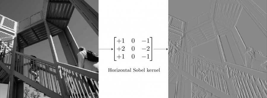
In flat areas, such as the sky, neighbouring pixels have similar values and the output is close to zero. At a vertical edge, the pixels on the left and right differ, and the kernel produces a large value. The kernel only looks at 3×3 patches, but applied across the whole image it finds edges everywhere.
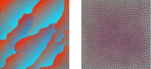
A CNN learns its kernels instead of having them designed. To see what they learned, researchers use feature visualization by optimization: start from random noise and adjust the image until a chosen filter is activated as strongly as possible. If the resulting image is full of edges, the filter is an edge detector. For the first layer of a trained network, the results look like this:
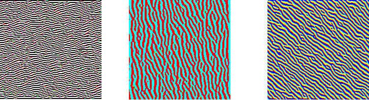
These filters respond to edges of different orientations and colours — low-level detectors, as expected. The outputs of a convolution are still images, laid out in the same order as the input, so convolutions can be stacked to detect more complex features. After the second and third convolution, the visualized features become textures:
But however deep the detectors go, a 3×3 kernel on its own still looks at a tiny patch: you cannot recognize a face in 3×3 pixels. This is where the receptive field comes in.
Receptive Field
The receptive field of a unit is the region of the original input that can influence it. In a CNN the spatial size shrinks from the input to the output while the number of channels grows, usually through strides or pooling. A strided convolution only keeps outputs at a fixed distance from each other:
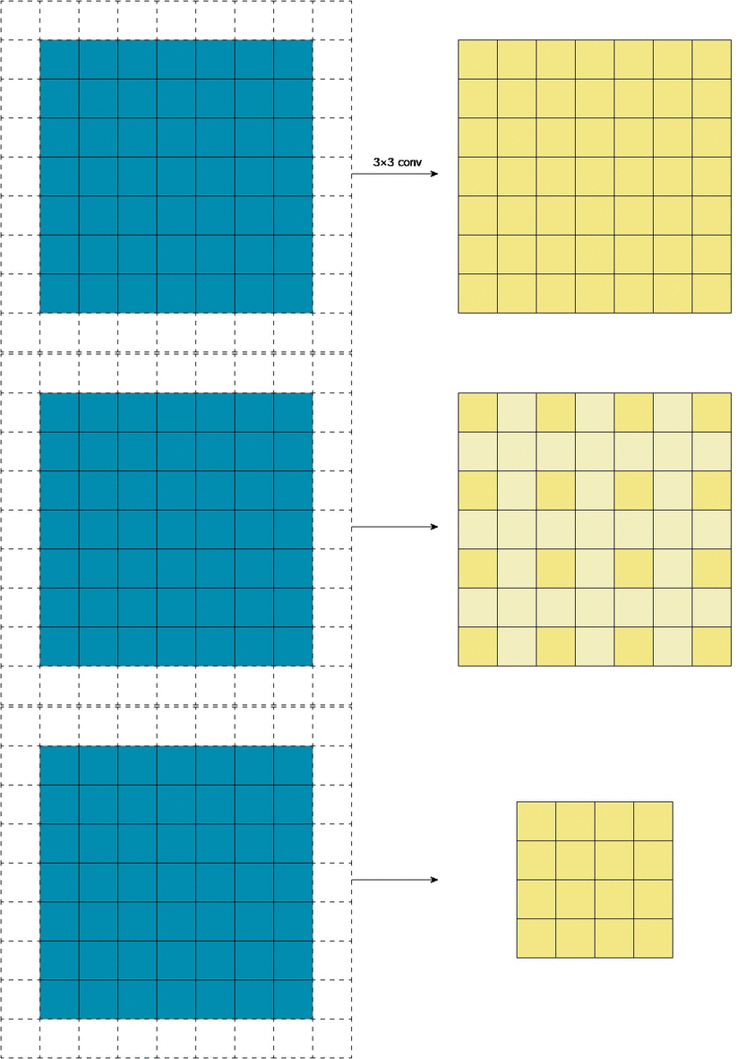
The next layer applies a kernel of the same 3×3 size to this smaller map, but now each of its inputs represents a larger area of the original image. The kernel has the same local view, yet its receptive field in the original image is larger:
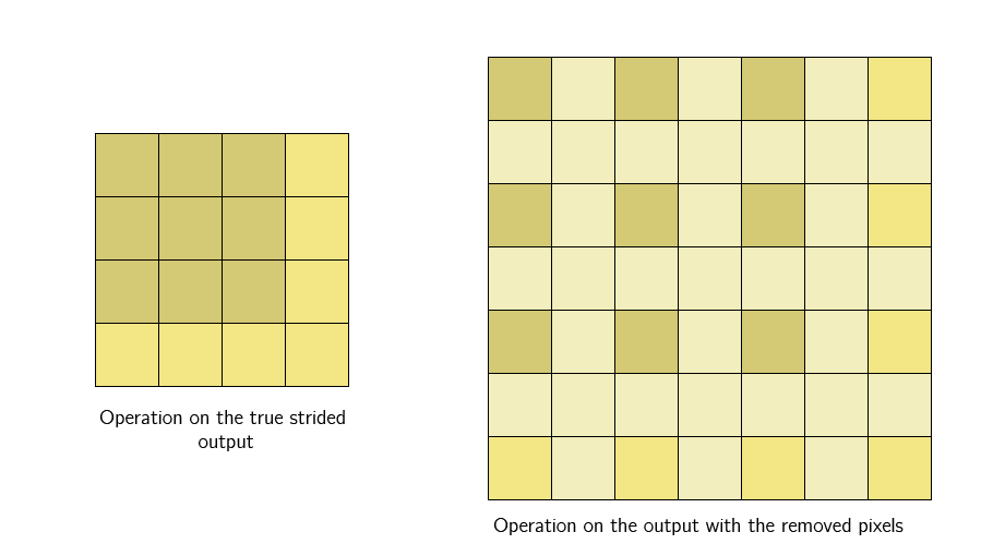
The receptive field is easy to compute: each layer adds (k − 1) times the product of the strides of all previous layers.
def receptive_field(layers):
    """layers: list of (kernel_size, stride). Returns receptive field after each layer."""
    rf, jump, out = 1, 1, []
    for k, s in layers:
        rf += (k - 1) * jump      # each layer adds (k - 1) steps of the current jump
        jump *= s                 # strides multiply the distance between outputs
        out.append(rf)
    return out

print("five 3x3 convs, stride 1:      ", receptive_field([(3, 1)] * 5))
print("3x3 conv + 2x2 pool, repeated: ", receptive_field([(3, 1), (2, 2)] * 4))
Output:
five 3x3 convs, stride 1:       [3, 5, 7, 9, 11]
3x3 conv + 2x2 pool, repeated:  [3, 4, 8, 10, 18, 22, 38, 46]
Without downsampling the receptive field grows slowly, by two pixels per layer. With pooling it roughly doubles at every stage. Dilated convolutions, which space out the kernel weights, are another way to grow the receptive field without reducing the resolution, and are popular in segmentation.
A growing receptive field lets each layer combine the features of the previous ones into more complex ones. In GoogLeNet, visualized below, the early layers detect edges and lines, layer mixed3a combines them into curves and textures, and after the next downsampling, layer mixed4a detects parts and patterns. By the last block the 224×224 input has shrunk to 7×7, so each position represents a 32×32 patch of the original image and responds to whole concepts such as birds or faces. The number of filters grows from 64 in the first layer to 1,024 in the last convolution.
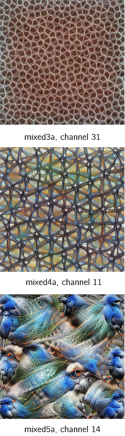
Finally, global pooling collapses each 7×7 map into a single value, so every channel becomes a detector whose receptive field is the entire image. Instead of an abstract combination of all pixels, as a fully connected network would learn, the CNN builds a strong visual hierarchy: low-level features combine into higher-level ones, layer by layer, until the network recognizes faces, birds and trees.
CNN Architecture and Famous Networks
A typical CNN for image classification repeats a simple pattern: a few convolution and activation layers, then downsampling, with the number of channels doubling every time the resolution halves.
| Stage | Layers | Output shape |
|---|---|---|
| Input | RGB image | 224 × 224 × 3 |
| Stem | 7×7 conv, stride 2, then 3×3 max pool, stride 2 | 56 × 56 × 64 |
| Stage 1–4 | Blocks of 3×3 convolutions; each new stage halves the size and doubles the channels | 56×56 → 28×28 → 14×14 → 7×7 |
| Head | Global average pooling, fully connected layer, softmax | number of classes |
The milestones of CNN design:
| Network | Year | Key idea |
|---|---|---|
| LeNet-5 | 1998 | Convolutions, pooling and a classifier, trained end to end for digit recognition |
| AlexNet | 2012 | A deep CNN trained on GPUs with ReLU and dropout; won ImageNet by a wide margin |
| VGG16 | 2014 | Only 3×3 convolutions stacked deep; simple and widely reused |
| GoogLeNet (Inception) | 2014 | Inception modules that run several kernel sizes in parallel; 1×1 convolutions to cut computation |
| ResNet | 2015 | Residual connections that make networks with over 100 layers trainable |
| MobileNet | 2017 | Depthwise separable convolutions for phones and embedded devices |
| EfficientNet | 2019 | Compound scaling of depth, width and resolution |
| ConvNeXt | 2022 | A pure CNN modernized with design choices from vision Transformers |
Two convolution variants from this table are worth knowing. A 1×1 convolution mixes channels at each pixel without looking at neighbours, and is used to reduce or expand the number of channels cheaply. A depthwise separable convolution splits a standard convolution into a per-channel spatial convolution and a 1×1 convolution, cutting the computation by roughly a factor of the kernel area.
Building a CNN in PyTorch
The example below trains a small CNN on the handwritten digits dataset that ships with scikit-learn: 1,797 grayscale images of 8×8 pixels. It prints the shape of the data after every layer, so you can follow how convolutions keep the size, pooling halves it, and the classifier turns the feature maps into 10 class scores:
import torch
import torch.nn as nn
from sklearn.datasets import load_digits
from sklearn.model_selection import train_test_split

torch.manual_seed(0)
digits = load_digits()                                  # 1,797 grayscale 8x8 images, 10 classes
X = torch.tensor(digits.images, dtype=torch.float32).unsqueeze(1) / 16.0   # (N, 1, 8, 8)
y = torch.tensor(digits.target)
X_train, X_test, y_train, y_test = train_test_split(X, y, test_size=0.25, stratify=y, random_state=0)

cnn = nn.Sequential(
    nn.Conv2d(1, 16, kernel_size=3, padding=1),         # (16, 8, 8)
    nn.ReLU(),
    nn.MaxPool2d(2),                                    # (16, 4, 4)
    nn.Conv2d(16, 32, kernel_size=3, padding=1),        # (32, 4, 4)
    nn.ReLU(),
    nn.MaxPool2d(2),                                    # (32, 2, 2)
    nn.Flatten(),                                       # 128
    nn.Linear(128, 10),
)

def train(model, epochs=30):
    opt = torch.optim.Adam(model.parameters(), lr=1e-2)
    loss_fn = nn.CrossEntropyLoss()
    for epoch in range(epochs):
        for i in range(0, len(X_train), 64):
            opt.zero_grad()
            loss = loss_fn(model(X_train[i:i + 64]), y_train[i:i + 64])
            loss.backward()
            opt.step()
    with torch.no_grad():
        return (model(X_test).argmax(1) == y_test).float().mean().item()

x = X_train[:1]
for layer in cnn:
    x = layer(x)
    print(f"{layer.__class__.__name__:>9}: {tuple(x.shape)}")

params = sum(p.numel() for p in cnn.parameters())
print(f"CNN: {params:,} parameters, test accuracy {train(cnn):.3f}")
Output:
   Conv2d: (1, 16, 8, 8)
     ReLU: (1, 16, 8, 8)
MaxPool2d: (1, 16, 4, 4)
   Conv2d: (1, 32, 4, 4)
     ReLU: (1, 32, 4, 4)
MaxPool2d: (1, 32, 2, 2)
  Flatten: (1, 128)
   Linear: (1, 10)
CNN: 6,090 parameters, test accuracy 0.982
With only 6,090 parameters the network classifies 98% of the unseen digits correctly. For real photos you would rarely train from scratch: the usual approach is transfer learning — take a CNN pretrained on ImageNet, such as a ResNet from torchvision.models, replace its final layer and fine-tune it on your images. Because the pretrained filters already detect general visual features, a few dozen to a few hundred images per class are often enough.
Applications of CNNs
- Image classification: deciding what an image shows, from product photos to plant diseases.
- Object detection: finding and labeling objects with bounding boxes, as in the R-CNN family and YOLO.
- Segmentation: classifying every pixel, for example with U-Net in medical imaging.
- Face recognition, OCR and video analysis.
- Beyond images: 1D convolutions for audio and time series, convolutions over spectrograms for speech, and convolutional layers inside image generation models such as the U-Nets of diffusion models.
CNN vs Vision Transformer
Since 2020, the Vision Transformer (ViT) has challenged CNNs. It cuts the image into patches, for example 16×16 pixels, and processes them with self-attention, so every patch can interact with every other one from the first layer on.
| CNN | Vision Transformer | |
|---|---|---|
| Built-in assumptions | Locality and weight sharing | Very few; learns spatial relations from data |
| Global context | Grows gradually with depth | Available in every layer |
| Data needed | Works well on small and medium datasets | Needs large datasets or pretraining |
| Compute | Efficient, scales linearly with the number of pixels | Attention scales quadratically with the number of patches |
| Typical use | Edge devices, real-time detection, medical imaging, smaller datasets | Large-scale pretraining, multimodal models |
The gap is smaller than it once seemed: ConvNeXt showed that a modernized CNN matches Transformers of the same size, and many current vision models are hybrids that use convolutions in the early layers and attention in the later ones.
Limitations and Adversarial Examples
Given their visual hierarchy, it is tempting to assume that CNNs see the way people do. They do handle real-world images remarkably well, but they fail in ways humans never would. The best-known example is adversarial examples: inputs changed very slightly, on purpose, to fool the model.
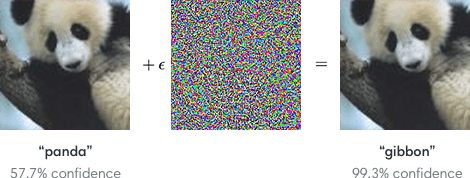
Adding a carefully computed pattern of noise, invisible to a person, makes the network change its answer from “panda” with 57.7% confidence to “gibbon” with 99.3% confidence. Such failures matter for self-driving cars, medical diagnosis and security systems, and defending against them is an active field of research. Other limitations include the need for large labeled datasets when training from scratch, sensitivity to changes in lighting, viewpoint and image quality that were not covered by the training data, and limited interpretability.
FAQ
What is a convolutional neural network in simple terms?
It is a neural network that looks at an image through many small windows. Each layer searches the image for simple patterns, and the next layers combine them into more complex ones, until the network recognizes whole objects.
What is the difference between a kernel and a filter?
A kernel is a 2D matrix of weights applied to one channel. A filter is a set of kernels, one per input channel, plus a bias; it produces one output channel. For single-channel inputs the two terms mean the same thing.
What does a pooling layer do?
It reduces the width and height of feature maps by summarizing small windows, usually with the maximum (max pooling) or the mean (average pooling). This lowers the computation and makes the network more tolerant to small shifts.
Why are CNNs better than fully connected networks for images?
Because they use far fewer parameters and build in two properties of images: nearby pixels are related, and the same pattern can appear anywhere. A fully connected layer on a 224×224 image would need billions of weights; a convolutional layer needs thousands.
Are CNNs still used now that there are vision Transformers?
Yes. CNNs are widely used in production, especially on mobile and edge devices, in real-time detection and in medical imaging, and modern CNNs such as ConvNeXt are competitive with Transformers of the same size.
See also: our breakdowns of AlexNet, VGG16 and ResNet, and our guide to backpropagation, the algorithm that trains CNN filters.