U-Net is considered one of the standard CNN architectures for image classification tasks, when we need not only to define the whole image by its class but also to segment areas of an image by class, i.e. produce a mask that will separate an image into several classes. The architecture consists of a contracting path to capture context and a symmetric expanding path that enables precise localization.
The network is trained in end-to-end fashion from very few images and outperforms the prior best method (a sliding-window convolutional network) on the ISBI challenge for segmentation of neuronal structures in electron microscopic stacks. Using the same network trained on transmitted light microscopy images (phase contrast and DIC), U-Net won the ISBI cell tracking challenge 2015 in these categories by a large margin. Moreover, the network is fast. Segmentation of a 512×512 image takes less than a second on a modern GPU.
Key Points
- Achieve Good performance on various real-life tasks especially biomedical application;
- Computational difficulty (how many and which GPUs you need, how long it will train);
- Uses a small number of data to achieve good results.
The U-net Architecture
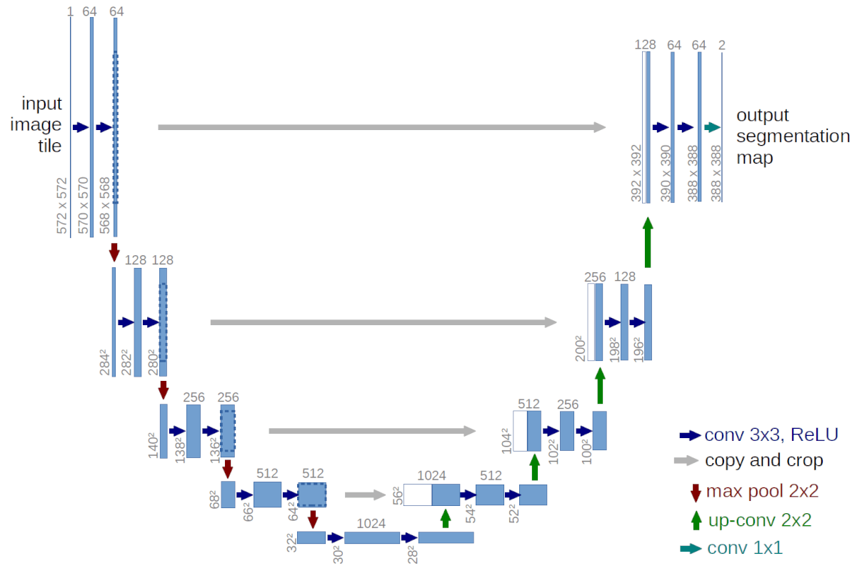
The network architecture is illustrated in Figure 1. It consists of a contracting path (left side) and an expansive path (right side). The contracting path follows the typical architecture of a convolutional network. It consists of the repeated application of two 3×3 convolutions (unpadded convolutions), each followed by a rectified linear unit (ReLU) and a 2×2 max pooling operation with stride 2 for downsampling.
At each downsampling step, feature channels are doubled. Every step in the expansive path consists of an upsampling of the feature map followed by a 2×2 convolution (up-convolution) that halves the number of feature channels, a concatenation with the correspondingly cropped feature map from the contracting path, and two 3×3 convolutions, each followed by a ReLU. The cropping is necessary due to the loss of border pixels in every convolution.
At the final layer, a 1×1 convolution is used to map each 64-component feature vector to the desired number of classes. In total the network has 23 convolutional layers.
Training
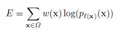
The input images and their corresponding segmentation maps are used to train the network with the stochastic gradient descent. Due to the unpadded convolutions, the output image is smaller than the input by a constant border width. A pixel-wise soft-max computes the energy function over the final feature map combined with the cross-entropy loss function. The cross-entropy that penalizes at each position is defined as:
The separation border is computed using morphological operations. The weight map is then computed as:
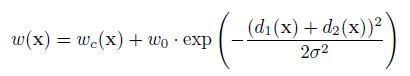
where wc is the weight map to balance the class frequencies, d1 denotes the distance to the border of the nearest cell and d2 denotes the distance to the border of the second nearest cell.
Use Cases and Implementation
U-net was applied to many real-time examples. Some of these are mentioned below:
- Ultrasound nerve classification competition on Kaggle and a couple of example kernels and code samples 1 2 3 4;
- Retina blood vessel segmentation working paper and code;
- Another U-net implementation with Keras;
- Applying small U-net for vehicle detection.
As we see from the example, this network is versatile and can be used for any reasonable image masking task. High accuracy is achieved, given proper training, adequate dataset and training time. If we consider a list of more advanced U-net usage examples we can see some more applied patters:
- Insights from satellite imagery competition;
- Another satellite imagery competition example;
- Lung cancer competition finalists also used U-net as part of their pipeline.
[Pytorch][Tensorflow][Keras]
Results
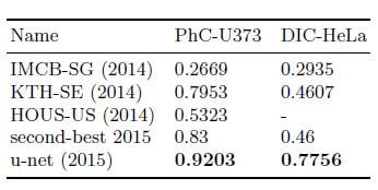
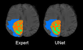
U-Net is applied to a cell segmentation task in light microscopic images. This segmentation task is part of the ISBI cell tracking challenge 2014 and 2015. The dataset PhC-U373 contains Glioblastoma-astrocytoma U373 cells on a polyacrylamide substrate recorded by phase contrast microscopy. It contains 35 partially annotated training images. Here U-Net achieved an average IOU (intersection over union) of 92%, which is significantly better than the second-best algorithm with 83% (see Fig 2). The second data set DIC-HeLa are HeLa cells on a flat glass recorded by differential interference contrast (DIC) microscopy [See below figures]. It contains 20 partially annotated training images. Here U-Net achieved an average IOU of 77.5% which is significantly better than the second-best algorithm with 46%.
The u-net architecture achieves outstanding performance on very different biomedical segmentation applications. It only needs very few annotated images and has a very reasonable training time of just 10 hours on NVidia Titan GPU (6 GB).


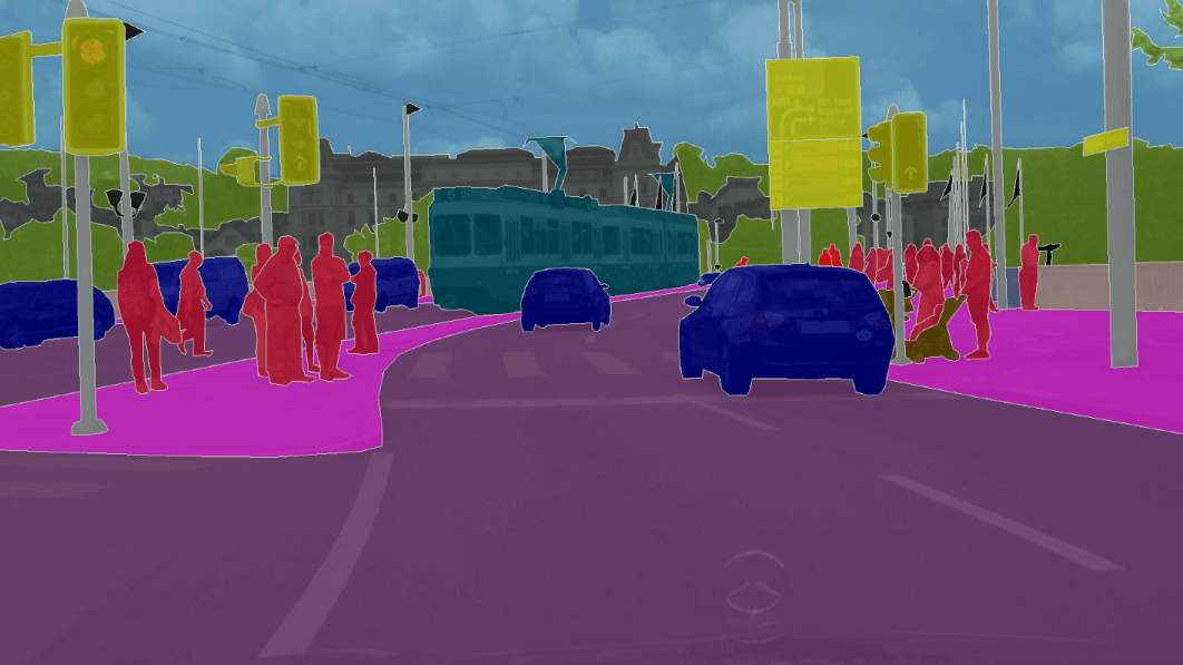
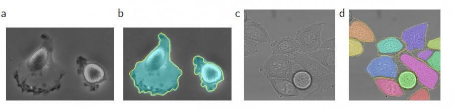
[…] U-Net semantic segmentation example on the right, Detectron model for instance segmentation on the left. […]