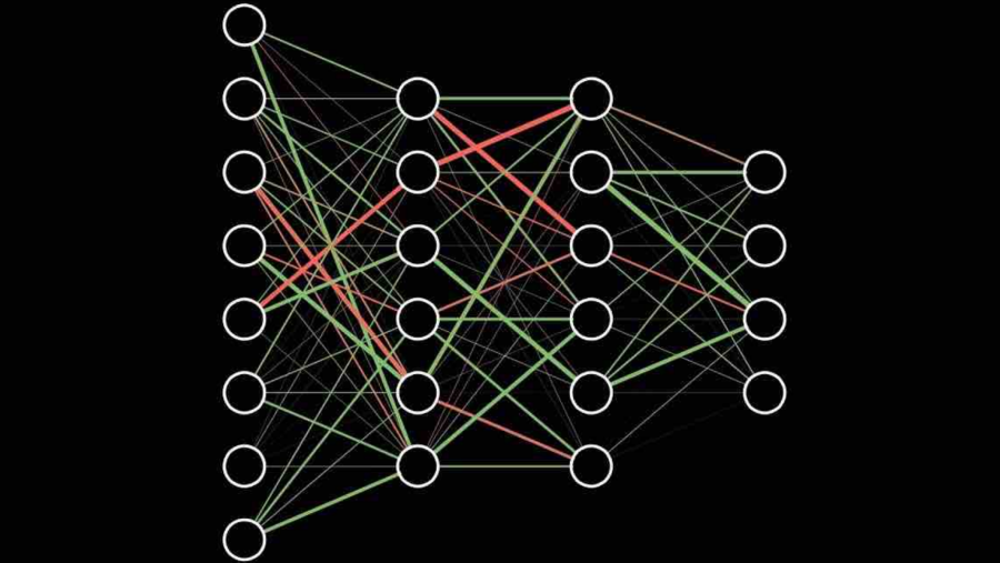
Deep learning is the part of machine learning that trains artificial neural networks with many layers to learn directly from raw data: pixels, sound waves, text. Instead of a programmer deciding which features matter, a deep network discovers them on its own, layer by layer. This idea is behind almost every AI breakthrough of the last fifteen years, from image recognition and speech assistants to ChatGPT, Claude, Gemini, image generators and AlphaFold.
This guide explains what deep learning is in simple terms, how a deep neural network works and learns, how deep learning differs from machine learning, the main types of deep learning models and where they are used. In a hands-on experiment we trained a linear model, a random forest, a shallow and a deep neural network and a convolutional network on the same clothing photos, from 1,000 to 60,000 examples, to see what depth really adds.
Key takeaways
- Deep learning is machine learning with neural networks that have several hidden layers. “Deep” refers to the number of layers, not to deep understanding.
- The main difference from classic machine learning: deep networks learn features from raw data themselves, so they need more data and computing power but scale much better.
- Training repeats four steps millions of times: forward pass, loss, backpropagation and a gradient descent update of the weights.
- Key architectures: convolutional networks for images, recurrent networks for sequences, transformers for language and most modern AI, and generative models such as diffusion models.
- In our experiment on 70,000 clothing photos, a convolutional network reached 92.1% accuracy against 87.8% for a random forest and 84.2% for a linear model, and its lead grew with more data. Simply adding fully connected layers helped only at the largest data size.
What is deep learning?
Deep learning is a machine learning method in which an artificial neural network with many layers learns to map inputs to outputs from examples. An input can be a photo, a recording or a sentence; the output can be a label (“cat”), a number (a price), a translation or a new image.
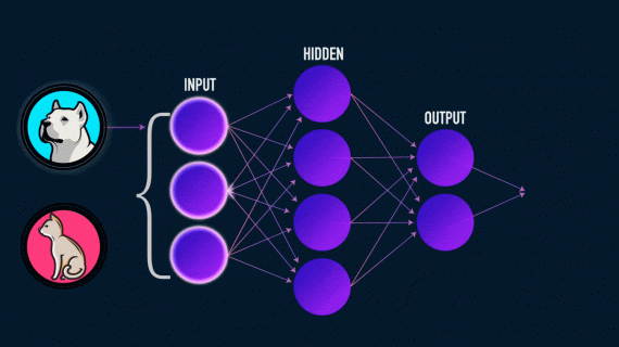
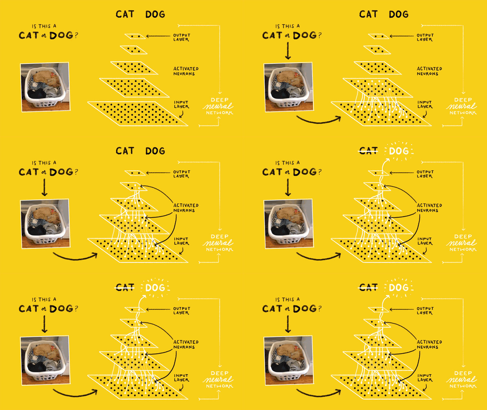
An artificial neural network is loosely inspired by the brain. It consists of simple units, artificial neurons, connected to each other. Each connection has a weight, a number that says how strongly one neuron influences the next. Neurons are organised in layers:
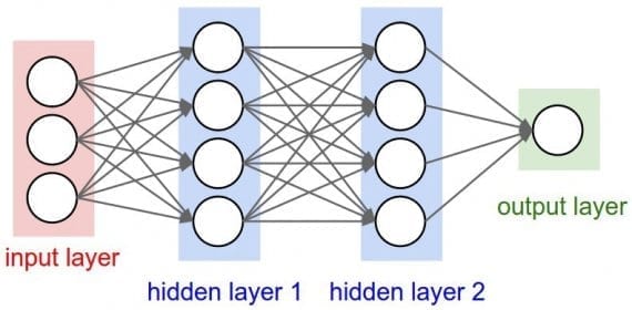
- the input layer receives the data, for example the pixel values of an image;
- hidden layers transform the data step by step;
- the output layer produces the answer.
A network with more than one hidden layer is called a deep neural network, and training it is deep learning. That is all “deep” means. Modern networks are far deeper than the textbook picture: ResNet, an image model from 2015, has up to 152 layers, and today’s large language models stack around a hundred transformer blocks with hundreds of billions of weights.
The reason depth matters is representation learning. Each layer builds on the one before it. In an image network, the first layers learn to detect edges and colour blobs, the middle layers combine them into textures and shapes, and the last layers recognise eyes, wheels or sleeves. Nobody programs these detectors: they emerge during training because they help the network reduce its errors.
Deep learning vs machine learning vs AI
The three terms are nested:
- Artificial intelligence (AI) is the broad goal of making machines perform tasks that require intelligence. Early AI used hand-written rules: chess programs and expert systems followed instructions written by people.
- Machine learning (ML) is the part of AI in which computers learn from data instead of following fixed rules. It includes linear models, decision trees, gradient boosting, support vector machines and neural networks.
- Deep learning (DL) is the part of machine learning that uses deep neural networks.
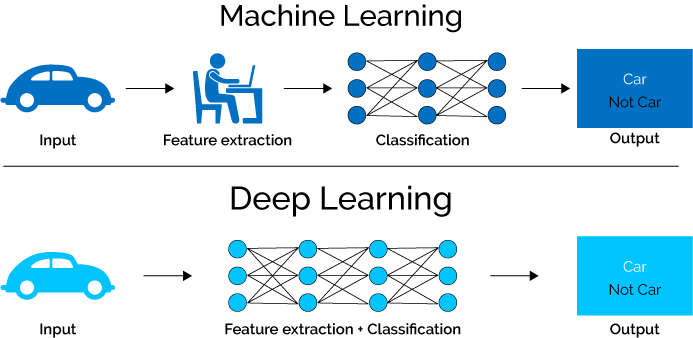
The practical difference between classic machine learning and deep learning is who designs the features:
| Classic machine learning | Deep learning | |
|---|---|---|
| Features | Designed by people (for example, “number of rooms”, “average purchase”) | Learned from raw data by the network |
| Best data type | Tables with meaningful columns | Images, audio, text, video and other raw signals |
| Data needed | Hundreds to thousands of examples can be enough | Usually thousands to billions of examples |
| Hardware | A normal CPU | GPUs or other accelerators for large models |
| Interpretability | Often easy to explain | Hard to explain: millions or billions of weights |
| Typical models | Linear regression, decision trees, random forests, gradient boosting | CNNs, RNNs, transformers, diffusion models |
Neither is better in general. On tabular business data such as customer records or transactions, gradient-boosted trees remain hard to beat. On images, speech and language, deep learning wins by a wide margin.
How deep learning works: an example
Imagine a service that predicts the price of a plane ticket. We train it with supervised learning: we show the network many past tickets with their real prices. The inputs are:
- the departure airport;
- the destination airport;
- the departure date;
- the airline.
The input layer has one neuron for each of these features (in practice, categories such as airports are turned into numbers first). The output layer has a single neuron: the predicted price. Between them are hidden layers.
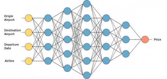
Each neuron in a hidden layer takes the outputs of the previous layer, multiplies each by the weight of its connection, adds them up together with a constant called the bias, and passes the sum through an activation function. The most common activation, ReLU, simply replaces negative numbers with zero. This non-linearity is essential: without it, any number of layers would collapse into one linear formula and the network could not learn complex relationships. For a step-by-step walkthrough with numbers and code, see our guide to how neural networks work.
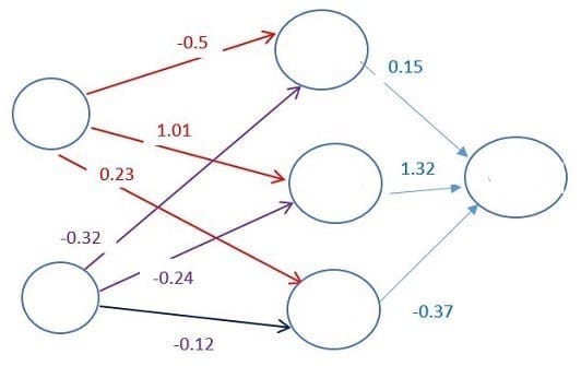
At the start, the weights are random, so the predictions are nonsense. The network becomes useful only after training, when the weights have been adjusted so that, for example, the departure date and the route strongly influence the price.
How a deep neural network learns
Training is the hardest part of deep learning, for two reasons: it needs a lot of data, and it needs a lot of computation. The process repeats the same loop many times:
- Forward pass. A batch of examples goes through the network, layer by layer, and produces predictions.
- Loss. A loss function measures how wrong the predictions are. For prices it can be the mean squared error; for classification, cross-entropy. Zero loss would mean perfect predictions on the training data.
- Backpropagation. Using the chain rule of calculus, backpropagation computes how the loss changes when each weight changes slightly: the gradient. It works backwards from the output layer to the input layer, which is where the name comes from.
- Gradient descent. Every weight moves a small step in the direction that reduces the loss. The size of the step is the learning rate. Modern training uses variants such as Adam or AdamW.
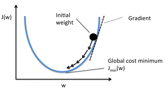
One pass through the whole training set is an epoch; the data is fed in small portions called batches. A model is trained for many epochs until the loss on new, held-out data stops improving. If the network keeps getting better on the training data but worse on new data, it is overfitting: memorising instead of learning. Techniques such as dropout, weight decay, data augmentation and simply more data fight it. You can read more about the optimisation itself in our guide to gradient descent.
All of this is automatic: frameworks such as PyTorch, JAX and TensorFlow compute the gradients for you, and GPUs perform the billions of multiplications in parallel. A network for a small task trains in minutes on a laptop; a frontier language model trains for months on tens of thousands of GPUs. See our guides to the best GPU for AI and to choosing between PyTorch and TensorFlow.
Types of deep learning models
- Feedforward networks (multilayer perceptrons). The basic architecture from the diagrams above, descended from Frank Rosenblatt’s perceptron of 1958. Every neuron connects to all neurons in the next layer.
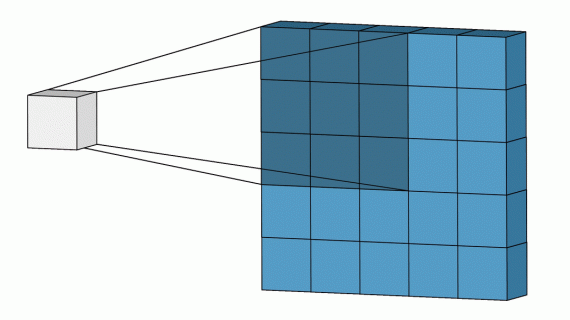
- Convolutional neural networks (CNNs). Use small filters that slide over an image, so the same pattern detector works everywhere in the picture. The standard for computer vision for a decade: AlexNet, VGG, ResNet.
- Recurrent neural networks (RNNs) and LSTM. Process sequences step by step with a memory of what came before. They dominated speech recognition and translation until about 2017 and are still used for some time series.
- Transformers. Introduced in 2017 in the paper “Attention Is All You Need”, they use attention to let every element of a sequence look at every other element in parallel. Transformers power large language models such as GPT, Claude, Gemini and Llama, and vision transformers compete with CNNs on images.
- Autoencoders and variational autoencoders. Compress data into a compact representation and reconstruct it; used for denoising, anomaly detection and as parts of image generators.
- Generative adversarial networks (GANs). Two networks compete: a generator creates fakes and a discriminator tries to spot them. They produced the first photorealistic generated faces.
- Diffusion models. Learn to turn random noise into images, video or audio by removing noise step by step. They are behind most modern image and video generators.
- Graph neural networks. Work on networks of connected objects such as molecules, social graphs or road maps.
Deep networks can be trained with any learning paradigm: supervised (labelled examples), unsupervised and self-supervised (learning from the structure of the data itself, such as predicting the next word, which is how language models are pretrained) and reinforcement learning (learning from rewards, used in AlphaGo and to fine-tune chatbots).
Experiment: does depth help?
To see what “deep” adds in practice, we trained five models on Fashion-MNIST, an open data set from Zalando Research (MIT licence) with 70,000 grayscale photos of clothing in 10 classes. It was created in 2017 as a harder replacement for the classic MNIST handwritten digits. Every model learned from the same 1,000, 5,000, 20,000 or 60,000 training images and was tested on 10,000 images it had never seen.
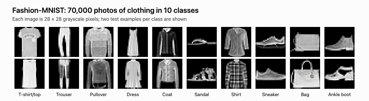
The models:
- Linear model: a neural network with no hidden layers, equivalent to multinomial logistic regression. It can only draw straight boundaries between classes.
- Random forest: 300 decision trees, a strong classic machine learning method that works on the raw pixels.
- Shallow network: one hidden layer of 256 neurons.
- Deep network: three hidden layers of 256 neurons.
- Convolutional network (CNN): two convolutional layers that learn local visual patterns, followed by a small fully connected part.
The code needs PyTorch, scikit-learn and NumPy. Download the four .gz files from the data/fashion folder of the Fashion-MNIST repository on GitHub into a data folder next to the script. All neural networks use the same training loop: Adam optimiser, batches of 64 images and at least 2,000 training steps.
import gzip
import time

import numpy as np
import torch
from torch import nn
from sklearn.ensemble import RandomForestClassifier

# 1. Fashion-MNIST: 70,000 grayscale 28x28 photos of clothes in 10 classes (MIT licence, Zalando Research)
def load(kind):
    with gzip.open(f"data/{kind}-images-idx3-ubyte.gz") as f:
        x = np.frombuffer(f.read(), np.uint8, offset=16).reshape(-1, 1, 28, 28) / 255.0
    with gzip.open(f"data/{kind}-labels-idx1-ubyte.gz") as f:
        y = np.frombuffer(f.read(), np.uint8, offset=8)
    return torch.tensor(x, dtype=torch.float32), torch.tensor(y, dtype=torch.long)

x_train, y_train = load("train")
x_test, y_test = load("t10k")
torch.manual_seed(0)

# 2. Four neural networks, from no hidden layers to a convolutional network
def make(name):
    if name == "Linear model (no hidden layers)":
        return nn.Sequential(nn.Flatten(), nn.Linear(784, 10))
    if name == "Shallow network (1 hidden layer)":
        return nn.Sequential(nn.Flatten(), nn.Linear(784, 256), nn.ReLU(), nn.Linear(256, 10))
    if name == "Deep network (3 hidden layers)":
        return nn.Sequential(nn.Flatten(), nn.Linear(784, 256), nn.ReLU(), nn.Linear(256, 256), nn.ReLU(),
                             nn.Linear(256, 256), nn.ReLU(), nn.Linear(256, 10))
    return nn.Sequential(                                   # convolutional network: learns visual features
        nn.Conv2d(1, 32, 3, padding=1), nn.ReLU(), nn.MaxPool2d(2),    # 28x28 -> 14x14
        nn.Conv2d(32, 64, 3, padding=1), nn.ReLU(), nn.MaxPool2d(2),   # 14x14 -> 7x7
        nn.Flatten(), nn.Dropout(0.3), nn.Linear(64 * 7 * 7, 128), nn.ReLU(), nn.Linear(128, 10))

def train(model, x, y, epochs):
    opt = torch.optim.Adam(model.parameters(), lr=1e-3)
    loss_fn = nn.CrossEntropyLoss()
    for epoch in range(epochs):
        model.train()
        for idx in torch.randperm(len(x)).split(64):        # mini-batches of 64 images
            loss = loss_fn(model(x[idx]), y[idx])           # forward pass: how wrong are we?
            opt.zero_grad()
            loss.backward()                                 # backpropagation: gradient of the loss
            opt.step()                                      # gradient descent step on all weights
    model.eval()
    with torch.no_grad():
        return (model(x_test).argmax(1) == y_test).float().mean().item()

# 3. Train every model on 1,000 to 60,000 examples and test on 10,000 images it has never seen
names = ["Linear model (no hidden layers)", "Shallow network (1 hidden layer)",
         "Deep network (3 hidden layers)", "Convolutional network (CNN)"]
for n in [1000, 5000, 20000, 60000]:
    x, y = x_train[:n], y_train[:n]
    epochs = max(10, int(np.ceil(2000 / (n / 64))))         # at least 2,000 training steps
    start = time.time()
    forest = RandomForestClassifier(300, n_jobs=-1, random_state=0).fit(x.flatten(1).numpy(), y.numpy())
    acc = forest.score(x_test.flatten(1).numpy(), y_test.numpy())
    print(f"{n:>6} examples  {'Random forest (classic ML)':34s} accuracy {acc:.3f}  {time.time() - start:5.0f} s")
    for name in names:
        start = time.time()
        model = make(name)
        acc = train(model, x, y, epochs)
        params = sum(p.numel() for p in model.parameters())
        print(f"{n:>6} examples  {name:34s} accuracy {acc:.3f}  {time.time() - start:5.0f} s  {params:,} weights")
1000 examples Random forest (classic ML) accuracy 0.800 2 s
1000 examples Linear model (no hidden layers) accuracy 0.794 18 s 7,850 weights
1000 examples Shallow network (1 hidden layer) accuracy 0.799 6 s 203,530 weights
1000 examples Deep network (3 hidden layers) accuracy 0.798 11 s 335,114 weights
1000 examples Convolutional network (CNN) accuracy 0.824 87 s 421,642 weights
5000 examples Random forest (classic ML) accuracy 0.837 8 s
5000 examples Linear model (no hidden layers) accuracy 0.818 2 s 7,850 weights
5000 examples Shallow network (1 hidden layer) accuracy 0.841 5 s 203,530 weights
5000 examples Deep network (3 hidden layers) accuracy 0.832 10 s 335,114 weights
5000 examples Convolutional network (CNN) accuracy 0.870 85 s 421,642 weights
20000 examples Random forest (classic ML) accuracy 0.864 36 s
20000 examples Linear model (no hidden layers) accuracy 0.836 2 s 7,850 weights
20000 examples Shallow network (1 hidden layer) accuracy 0.871 8 s 203,530 weights
20000 examples Deep network (3 hidden layers) accuracy 0.862 13 s 335,114 weights
20000 examples Convolutional network (CNN) accuracy 0.898 123 s 421,642 weights
60000 examples Random forest (classic ML) accuracy 0.878 133 s
60000 examples Linear model (no hidden layers) accuracy 0.842 7 s 7,850 weights
60000 examples Shallow network (1 hidden layer) accuracy 0.881 23 s 203,530 weights
60000 examples Deep network (3 hidden layers) accuracy 0.889 42 s 335,114 weights
60000 examples Convolutional network (CNN) accuracy 0.921 387 s 421,642 weightsThe first line’s 18 seconds for the linear model include PyTorch’s one-time start-up; on later runs it trains in a few seconds.
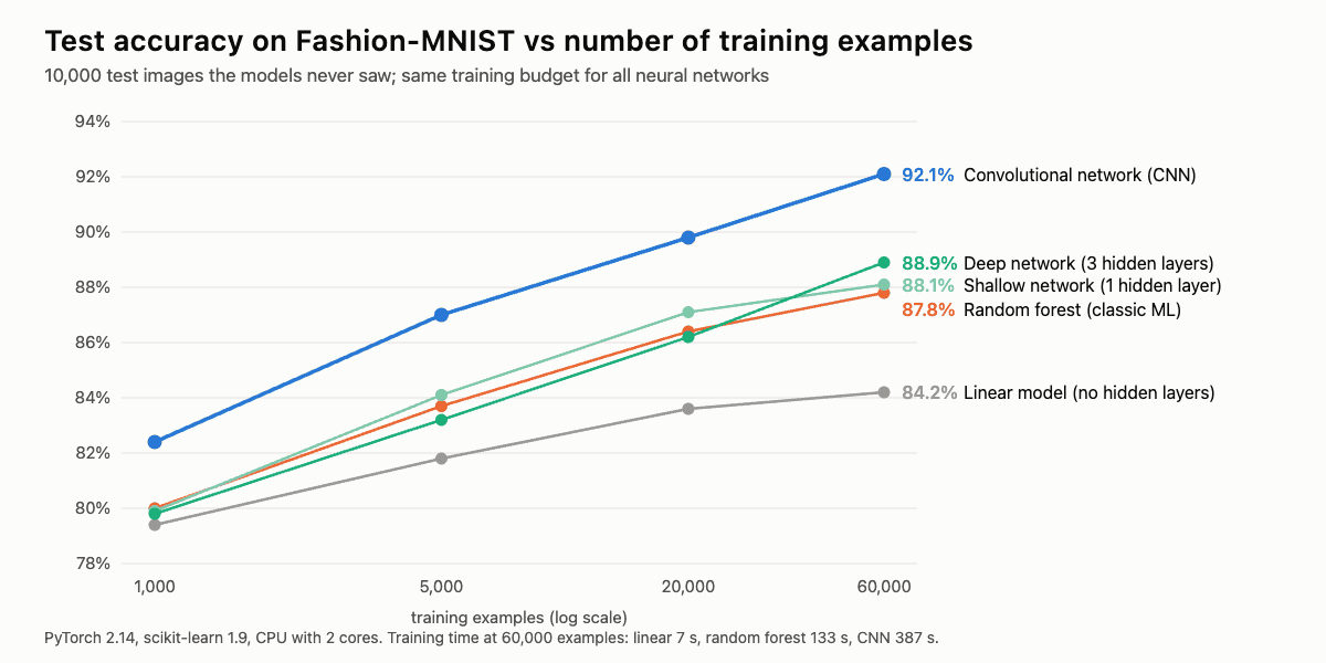
What the experiment shows:
- The right architecture beats extra layers. The convolutional network won at every data size, reaching 92.1% accuracy against 87.8% for the random forest. Its error rate on the full data set, 7.9%, is about a third lower than the forest’s 12.2%. The CNN wins because it is built for images: the same small filters scan the whole picture and learn edges, textures and shapes.
- More layers need more data. The fully connected network with three hidden layers was slightly worse than the shallow one with 1,000 to 20,000 examples and pulled ahead only at 60,000 (88.9% against 88.1%). Depth adds weights, 335,000 instead of 204,000, and weights need examples to be tuned.
- Deep learning scales with data, simple models plateau. Going from 20,000 to 60,000 examples improved the linear model by only 0.6 points, while the CNN gained 2.3 points. This is the typical pattern behind modern AI: give deep models more data and computing power, and they keep improving.
- The price is computation. On a two-core CPU the CNN needed 387 seconds on the full data set, three times longer than the forest and 55 times longer than the linear model. On a GPU the same training takes seconds, which is why GPUs became the engine of deep learning.
Specialised architectures go much further: well-tuned CNNs and vision transformers with data augmentation reach about 94% to 96% on Fashion-MNIST. The lesson holds for every domain: deep learning works best when the architecture matches the structure of the data, convolutions for images and attention for language, and when there is enough data to train it.
A short history of deep learning
| Year | Milestone |
|---|---|
| 1943 | Warren McCulloch and Walter Pitts describe a mathematical model of a neuron. |
| 1958 | Frank Rosenblatt builds the perceptron, a single-layer network that learns from examples. |
| 1986 | David Rumelhart, Geoffrey Hinton and Ronald Williams popularise backpropagation for training multilayer networks. |
| 1989–1998 | Yann LeCun develops convolutional networks (LeNet) that read handwritten digits on bank cheques. |
| 1997 | Sepp Hochreiter and Jürgen Schmidhuber publish LSTM. |
| 2006 | Hinton’s team shows how to train deep belief networks layer by layer; the term “deep learning” spreads. |
| 2012 | AlexNet wins the ImageNet challenge with a top-5 error of 15.3% against 26.2% for the runner-up, trained on two gaming GPUs. The deep learning boom begins. |
| 2014–2015 | GANs are invented; ResNet trains networks with more than 100 layers and beats the human benchmark on ImageNet. |
| 2016 | DeepMind’s AlphaGo defeats Go champion Lee Sedol. |
| 2017 | The transformer architecture is published. |
| 2018 | Yoshua Bengio, Geoffrey Hinton and Yann LeCun receive the Turing Award for deep learning. |
| 2020 | AlphaFold 2 predicts protein structures with accuracy close to experiments. |
| 2022 | ChatGPT brings large language models to the public; diffusion models make image generation mainstream. |
| 2024 | Nobel Prizes: physics to John Hopfield and Geoffrey Hinton for foundational work on neural networks; chemistry partly to Demis Hassabis and John Jumper for AlphaFold. |
| 2025–2026 | Reasoning models that “think” before answering, AI agents that use tools, and multimodal models that work with text, images, audio and video at once. |
Three things came together to make deep learning work after decades of slow progress: large labelled data sets such as ImageNet, cheap parallel computing on GPUs, and better training techniques (ReLU activations, good weight initialisation, dropout, batch normalisation, residual connections and the Adam optimiser).
Deep learning applications and examples
- Language: chatbots and assistants, translation, summarisation, search, code generation.
- Computer vision: face unlock on phones, photo search, medical image analysis, quality control in factories, self-driving and driver-assistance systems.
- Speech: voice assistants, automatic subtitles and transcription (for example, OpenAI’s Whisper), realistic speech synthesis.
- Generative AI: images, video, music and 3D models from text prompts.
- Science and medicine: protein structure prediction, drug discovery, weather forecasting (Google DeepMind’s GraphCast and similar models rival traditional forecasts), materials discovery.
- Recommendations and ads: the feeds of video, music and shopping platforms are ranked by deep networks; see our guide to recommender systems.
- Games and robotics: AlphaGo and AlphaZero, robot grasping and walking, warehouse automation.
Limitations
- Data hunger. Deep networks need many examples, and the examples must be representative. A model trained on biased data reproduces the bias.
- Compute and energy. Training large models costs millions of dollars and consumes a lot of electricity.
- Black box. It is hard to explain why a network made a particular decision, which is a problem in medicine, finance and law. Interpretability research is trying to open the box.
- Brittleness. Small, carefully chosen changes to an input (adversarial examples) can fool a network, and models can fail on data that differs from what they saw in training.
- Confident mistakes. Language models can “hallucinate” plausible but false statements.
How to start learning deep learning
- Learn Python and the basics of NumPy. Some linear algebra, derivatives and probability help but can be learned along the way.
- Understand classic machine learning first: training and test sets, overfitting, evaluation metrics.
- Pick a framework. PyTorch is the most widely used in research and increasingly in industry.
- Take a practical course: fast.ai’s “Practical Deep Learning for Coders”, Andrew Ng’s Deep Learning Specialization, the free interactive book “Dive into Deep Learning” (d2l.ai) or Stanford’s CS231n lectures.
- Build projects: start with a small image classifier like the one in our experiment, then fine-tune a pretrained model on your own data. Fine-tuning is how most real-world deep learning is done today.
FAQ
What is deep learning in simple words?
Deep learning is a way of teaching computers by example using artificial neural networks with many layers. You show the network thousands of examples, it guesses, measures its mistakes and slightly adjusts millions of internal numbers, until it gets the answers right on examples it has never seen.
Why is it called deep learning?
Because the neural networks have many layers stacked on top of each other: they are “deep”. A network with one hidden layer is shallow; a network with two or more hidden layers is deep. Modern models have dozens to hundreds of layers.
What is the difference between deep learning and machine learning?
Deep learning is a subset of machine learning. Classic machine learning usually relies on features that people design and works well on tabular data; deep learning learns the features itself from raw data such as images, sound and text, and needs more data and computing power.
Is ChatGPT deep learning?
Yes. ChatGPT, Claude, Gemini and other chatbots are large language models: deep neural networks based on the transformer architecture, trained on huge amounts of text and then fine-tuned with human feedback and reinforcement learning.
What are examples of deep learning?
Face recognition on phones, voice assistants, machine translation, chatbots, image and video generators, recommendation feeds, medical image analysis, self-driving car perception and AlphaFold’s protein structure predictions.
Do I need a GPU for deep learning?
Not to start. Small networks like the ones in our experiment train on an ordinary CPU in minutes. For larger models and image or language tasks, a GPU speeds up training by tens of times, and cloud GPUs can be rented by the hour.