A generative adversarial network (GAN) is a generative model made of two neural networks trained against each other. The generator turns random noise into fake data, such as images; the discriminator looks at real and fake examples and tries to tell them apart. Each network improves by exploiting the weaknesses of the other, and if training goes well, the generator ends up producing samples the discriminator cannot distinguish from real ones. GANs were introduced by Ian Goodfellow and colleagues in 2014; Yann LeCun called adversarial training “the most interesting idea in the last 10 years in machine learning”. They powered the first photorealistic face generators, StyleGAN and image-to-image translation, and they are still used for super-resolution, fast image generation and as a component of diffusion pipelines.
This guide explains how GANs work: the generator and discriminator, the adversarial training loop, the minimax loss, a complete PyTorch implementation with real results, why GANs are hard to train and how to fix it, the main architectures from DCGAN to StyleGAN, and how GANs compare with VAEs and diffusion models.
Key takeaways
- Two networks: the generator maps noise
zto a fake sampleG(z); the discriminator outputs the probabilityD(x)that its input is real. - Adversarial training: the discriminator is trained to label real data 1 and fakes 0, the generator to make the discriminator say 1 for its fakes.
- Minimax game: at the ideal equilibrium the generator reproduces the data distribution and the discriminator outputs 0.5 everywhere.
- Hard to train: typical failures are mode collapse, vanishing generator gradients and oscillation; WGAN, spectral normalization and careful hyperparameters help.
- Today: diffusion models have overtaken GANs for most image generation, but GANs remain the fastest generators and their adversarial loss is built into many modern systems.
What Is a Generative Adversarial Network?
Most neural networks are trained to recognize things: is this email spam, what object is in this photo. A generative model is trained to create things — new examples that look as if they came from the training data. The potential of GANs is huge because they can learn to imitate almost any data distribution: images, music, speech, video or tabular records.
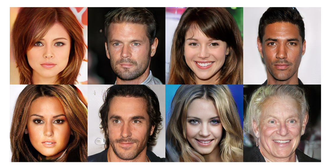
The GAN was proposed in the 2014 paper “Generative Adversarial Nets” by Ian Goodfellow and co-authors at the University of Montreal, including Yoshua Bengio. Its idea is to replace a hand-designed measure of “realism” with a second neural network that learns what realism means. Within a few years GANs went from blurry digits to photographs of people who do not exist:
The Forger and the Shop Owner
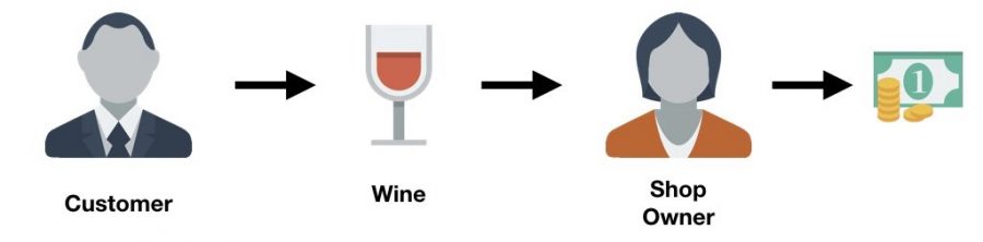
The easiest way to understand a GAN is an analogy. Imagine a shop that buys wine from suppliers and resells it. Honest suppliers bring real wine, and the shop owner pays for it:
But there are also forgers who try to sell fake wine. The shop owner has to learn to tell fake bottles from genuine ones and reject them:
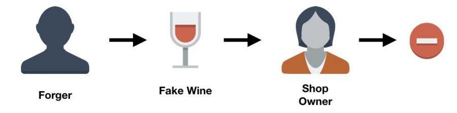
At first the forgers make many mistakes and the owner catches them easily. By trial and error, the forgers learn to imitate real wine better, and eventually some fakes get through. The owner, in turn, gets feedback about the fakes that slipped past and becomes better at spotting them. Each side keeps improving in response to the other, in a constant escalation.
A GAN is exactly this setup. The forger is the generator, which turns a random noise vector — its “inspiration” — into fake data. The shop owner is the discriminator, which sees both real data from the training set and fakes from the generator, and decides which is which:
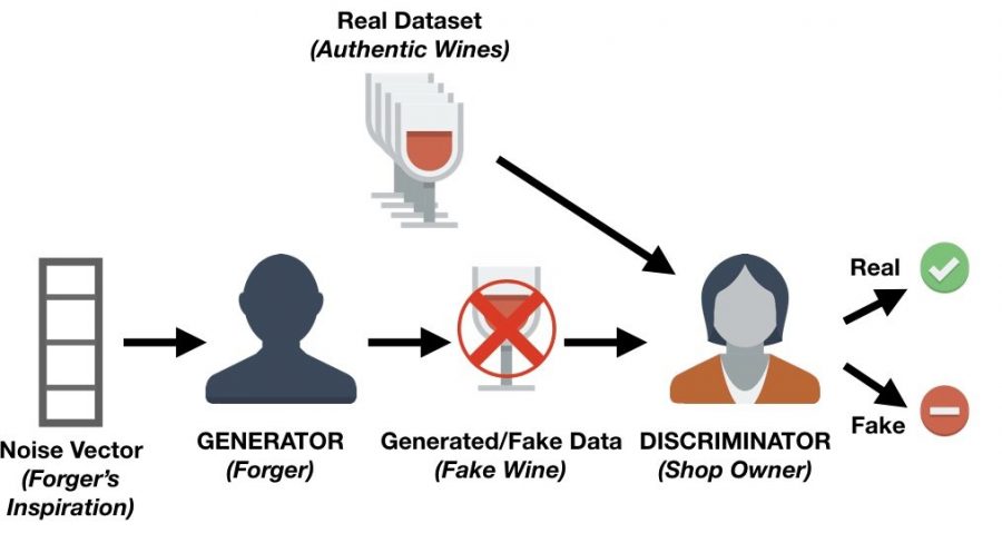
The same story is often told with a counterfeiter and the police: the counterfeiter learns to print convincing banknotes, the police learn to detect them, and both are constantly learning.
Discriminative vs Generative Models
The discriminator and the generator represent two kinds of models.
- A discriminative model predicts a label from features. A spam filter reads the words of an email
xand estimatesp(y | x), the probability that it is spam. Discriminative models learn the boundary between classes. - A generative model learns where the features come from: the distribution
p(x), orp(x | y)for a given class. It can produce new examples, and it can also be used for classification. Generative models learn the distribution of each class.
A GAN trains a generative model with the help of a discriminative one. The discriminator is an ordinary binary classifier — real or fake — and its judgments are the only training signal the generator ever receives. The generator never sees a real example directly.
How a GAN Works
Suppose we want to generate handwritten digits like those in the MNIST dataset. One training step goes like this:
- The generator takes a vector of random numbers
z, sampled from a normal distribution, and returns an imageG(z). - The fake image is fed to the discriminator together with real images from the dataset.
- The discriminator returns a probability between 0 and 1 for each image: 1 means real, 0 means fake.
- The discriminator is updated to give real images higher scores and fakes lower ones.
- The generator is updated, through the discriminator, to make its fakes score higher.
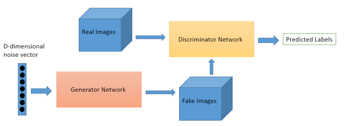
There is a double feedback loop: the discriminator learns from the ground truth of which images are real, and the generator learns from the discriminator. For images, the discriminator is usually a convolutional network that downsamples the image into a single probability, while the generator works like a convolutional network in reverse: it starts from a noise vector and upsamples it, typically with transposed convolutions, into a full image.
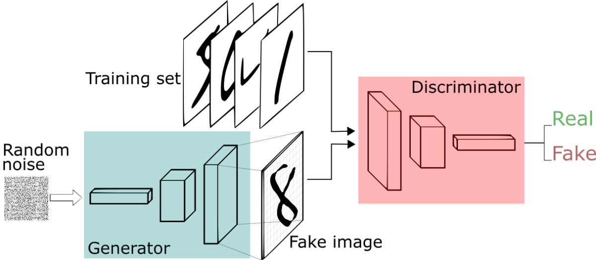
Both networks are trained with backpropagation and gradient descent. The gradient for the generator flows backward through the discriminator into the generator, which is how the generator learns which changes to its output make it look more real. While one network is updated, the other is held fixed.
The GAN Loss Function
Formally, the two networks play a two-player minimax game with the value function
minG maxD V(D, G) = Ex~data[ log D(x) ] + Ez~p(z)[ log(1 − D(G(z))) ]
The discriminator maximizes it: it wants D(x) close to 1 for real data and D(G(z)) close to 0 for fakes. This is simply the binary cross-entropy loss of a real-vs-fake classifier. The generator minimizes it by pushing D(G(z)) towards 1.
Goodfellow and co-authors showed that for a fixed generator the best discriminator is D*(x) = pdata(x) / (pdata(x) + pg(x)), and that with this discriminator the game minimizes the Jensen–Shannon divergence between the real distribution and the generator distribution. The global optimum is reached when the generator reproduces the data distribution exactly: then D(x) = 0.5 everywhere, and the discriminator can only guess.
In practice the generator does not minimize log(1 − D(G(z))). Early in training the discriminator rejects fakes easily, this term saturates, and its gradient vanishes. Instead, the generator maximizes log D(G(z)) — the non-saturating loss, which is the same as training it with binary cross-entropy against the label “real”. This is what the code below does.
Building a GAN in PyTorch
The GAN below learns to generate the 8×8 handwritten digits that ship with scikit-learn. Both networks are small fully connected networks; the generator ends with tanh, so the images are scaled to the range −1 to 1. Each step updates the discriminator on a batch of real and fake images, then updates the generator. At the end, a classifier trained on real digits labels 2,000 generated images to see which digits the generator produces:
import torch
import torch.nn as nn
from sklearn.datasets import load_digits

torch.manual_seed(0)
X = torch.tensor(load_digits().data, dtype=torch.float32) / 8.0 - 1.0   # 1,797 images, pixels in [-1, 1]
latent_dim = 16

generator = nn.Sequential(                      # noise z -> fake image
    nn.Linear(latent_dim, 128), nn.LeakyReLU(0.2),
    nn.Linear(128, 256), nn.LeakyReLU(0.2),
    nn.Linear(256, 64), nn.Tanh(),
)
discriminator = nn.Sequential(                  # image -> logit of "real"
    nn.Linear(64, 256), nn.LeakyReLU(0.2),
    nn.Linear(256, 128), nn.LeakyReLU(0.2),
    nn.Linear(128, 1),
)
opt_g = torch.optim.Adam(generator.parameters(), lr=2e-4, betas=(0.5, 0.999))
opt_d = torch.optim.Adam(discriminator.parameters(), lr=2e-4, betas=(0.5, 0.999))
bce = nn.BCEWithLogitsLoss()

for epoch in range(1, 301):
    for real in X[torch.randperm(len(X))].split(64):
        n = len(real)
        fake = generator(torch.randn(n, latent_dim))

        # 1) Discriminator step: real images -> 1, fake images -> 0
        d_loss = (bce(discriminator(real), torch.ones(n, 1)) +
                  bce(discriminator(fake.detach()), torch.zeros(n, 1)))
        opt_d.zero_grad()
        d_loss.backward()
        opt_d.step()

        # 2) Generator step: try to make the discriminator say 1 for fakes
        g_loss = bce(discriminator(fake), torch.ones(n, 1))
        opt_g.zero_grad()
        g_loss.backward()
        opt_g.step()

    if epoch in (1, 10, 100, 300):
        with torch.no_grad():
            d_real = torch.sigmoid(discriminator(X)).mean()
            d_fake = torch.sigmoid(discriminator(generator(torch.randn(1000, latent_dim)))).mean()
        print(f"epoch {epoch:3d}: D loss {d_loss:.2f}, G loss {g_loss:.2f}, "
              f"D(real) {d_real:.2f}, D(fake) {d_fake:.2f}")

# Which digits does the generator produce? Label 2,000 samples with a classifier trained on real digits
from sklearn.svm import SVC
digits = load_digits()
classifier = SVC(gamma=0.001).fit(digits.data, digits.target)
with torch.no_grad():
    samples = ((generator(torch.randn(2000, latent_dim)) + 1) * 8).clamp(0, 16).numpy()   # back to 0..16
counts = torch.bincount(torch.tensor(classifier.predict(samples)), minlength=10)
print("generated digits per class:", counts.tolist())
Output (about a minute on a CPU):
epoch   1: D loss 1.12, G loss 0.58, D(real) 0.75, D(fake) 0.58
epoch  10: D loss 0.78, G loss 1.45, D(real) 0.67, D(fake) 0.38
epoch 100: D loss 1.50, G loss 2.30, D(real) 0.64, D(fake) 0.30
epoch 300: D loss 1.16, G loss 1.78, D(real) 0.65, D(fake) 0.35
generated digits per class: [138, 162, 137, 309, 145, 247, 92, 189, 254, 327]
Notice that the losses do not steadily decrease, as they would in ordinary training: each network’s progress makes the other’s job harder, so the numbers fluctuate. The discriminator stays uncertain, scoring real images around 0.65 and fakes around 0.35, far from a clean 1 and 0. Here is what the generator produces from the same 12 noise vectors as training goes on:
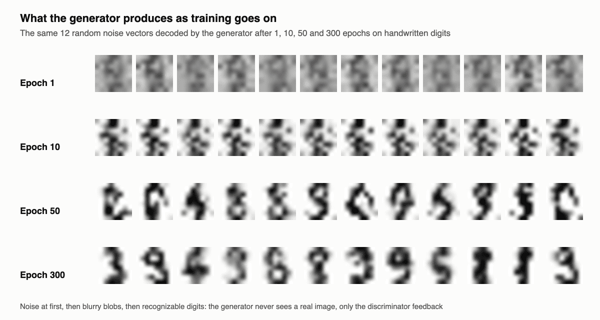
After one epoch the output is grey noise; after ten, blobs with a vague digit-like structure; after fifty, rough shapes; after three hundred, recognizable digits such as 3, 9, 4 and 5. The classifier finds all ten digits among the generated images, but not in equal numbers:
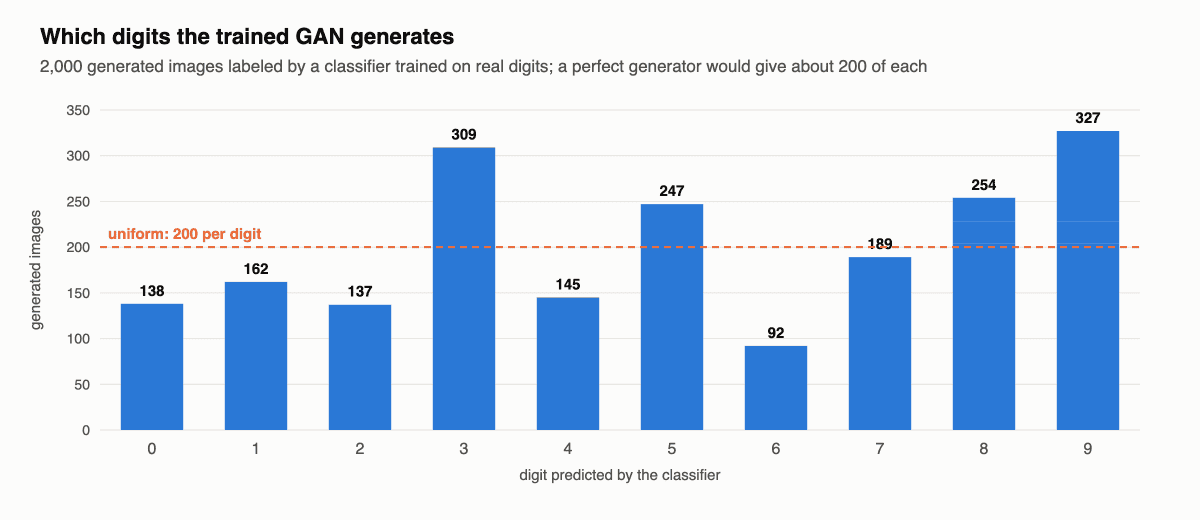
Threes and nines are produced more than three times as often as sixes. This uneven coverage is a mild form of the most famous GAN problem, mode collapse.
Why GANs Are Hard to Train
Training a GAN means finding an equilibrium between two networks rather than minimizing a single loss, and that makes it fragile:
- Mode collapse. The generator finds a few outputs that fool the discriminator and keeps producing them, ignoring the rest of the data distribution — for example, generating only a few kinds of digits or faces. In the extreme case every noise vector maps to nearly the same image.
- Vanishing gradients. If the discriminator becomes too good, it outputs values very close to 0 for every fake, and the generator receives almost no useful gradient.
- Oscillation and non-convergence. The two networks can chase each other in circles without settling, and sample quality may improve and then degrade again.
- No reliable loss curve. The losses do not tell you how good the samples are, so progress has to be judged by looking at samples or by metrics such as the Fréchet Inception Distance (FID).
- Sensitivity to hyperparameters. Learning rates, architectures and the balance between the two networks all matter, and settings that work on one dataset often fail on another.
Either network can overpower the other. If the discriminator is too strong, the generator stops learning; if the generator is too strong, it exploits the discriminator’s blind spots and produces fakes the discriminator wrongly accepts. GANs also take a long time to train: hours on a GPU for small images, days or weeks for high-resolution ones.
Tips for Training GANs
- Use Adam with a learning rate of 2e-4 and β₁ = 0.5, the defaults from DCGAN that the code above uses.
- Scale images to [−1, 1] and end the generator with
tanh; use LeakyReLU in the discriminator. - Train against a fixed opponent: freeze the generator while updating the discriminator and vice versa, and call
detach()on fakes in the discriminator step. - Use the non-saturating generator loss, or the Wasserstein loss with a gradient penalty (WGAN-GP), which gives useful gradients even when the discriminator is strong.
- Constrain the discriminator with spectral normalization, which became standard in large GANs, or use one-sided label smoothing (real labels of 0.9 instead of 1).
- Watch the samples, not the losses, and keep a fixed batch of noise vectors to compare outputs across training, as in the figure above.
- Measure quality with FID, which compares statistics of real and generated images, and check diversity separately to catch mode collapse.
GAN Architectures: DCGAN, StyleGAN, CycleGAN and More
| Model | Year | Key idea |
|---|---|---|
| GAN | 2014 | Generator and discriminator trained in a minimax game |
| Conditional GAN | 2014 | Both networks receive a label, so you can choose what to generate |
| DCGAN | 2015 | Convolutional architecture and training rules that made GANs stable on images |
| Pix2pix | 2016 | Conditional GAN for paired image-to-image translation: sketches to photos, maps to aerial images |
| CycleGAN | 2017 | Image-to-image translation without paired examples, using a cycle-consistency loss: horses to zebras, summer to winter |
| WGAN, WGAN-GP | 2017 | Wasserstein distance instead of Jensen–Shannon divergence, for more stable training and meaningful loss curves |
| Progressive GAN | 2017 | Starts at low resolution and adds layers during training; first 1024×1024 faces |
| BigGAN | 2018 | Large-scale class-conditional GAN on ImageNet |
| StyleGAN, StyleGAN2, StyleGAN3 | 2018–2021 | Style-based generator that controls coarse and fine features separately; photorealistic faces |
| GigaGAN | 2023 | Text-to-image GAN with a billion parameters, generating images in a fraction of a second |
The pictures of non-existent celebrities at the top of this guide come from Nvidia’s Progressive GAN. Its successor, StyleGAN, powered the well-known “this person does not exist” demos and is still used for face editing and avatars.
GAN vs VAE vs Diffusion Models
It is useful to compare GANs with autoencoders. An autoencoder compresses its input into a small latent vector with an encoder and reconstructs it with a decoder:
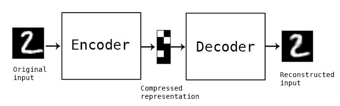
A variational autoencoder adds a constraint that makes its latent space a smooth normal distribution, so its decoder can generate new data like a GAN generator. But VAEs are trained to reconstruct their inputs on average, which makes their samples blurry, while a GAN generator is trained only to fool a discriminator and produces sharper details. Diffusion models, which learn to remove noise step by step, now produce the highest-quality and most diverse images.
| GAN | VAE | Diffusion model | |
|---|---|---|---|
| Training | Adversarial game, unstable | Single loss (ELBO), stable | Single denoising loss, stable |
| Sample quality | Sharp | Often blurry | Sharp |
| Diversity | Prone to mode collapse | Good | Best |
| Generation speed | One forward pass, real time | One forward pass | Many steps, unless distilled |
| Encoder for real images | No (needs GAN inversion) | Yes | Indirect |
Since 2021, when OpenAI researchers showed that diffusion models beat GANs on image synthesis benchmarks, most new text-to-image systems have been diffusion-based. GANs did not disappear, though. Adversarial losses are used to train the autoencoders behind latent diffusion models, to sharpen super-resolution models, and to distill slow diffusion models into fast generators that need only one to four steps, as in adversarial diffusion distillation.
Applications of GANs
- Image synthesis: realistic faces, objects and scenes; avatars and game assets.
- Image-to-image translation: sketches to photos, day to night, style transfer, colorization (pix2pix, CycleGAN).
- Super-resolution and restoration: sharpening and upscaling photos and video, and repairing old images, for example with ESRGAN.
- Image editing and inpainting: changing age, expression or lighting in a face, filling in missing regions.
- Data augmentation and synthetic data: generating extra training examples, for instance rare cases in medical imaging, or privacy-preserving synthetic tables.
- Audio and speech: GAN vocoders such as HiFi-GAN turn spectrograms into natural-sounding speech in real time.
The same technology makes deepfakes possible, which is why detecting GAN-generated images and video has become a research field of its own.
FAQ
What is a GAN in simple terms?
It is a pair of neural networks that compete. One creates fake data, the other tries to spot the fakes. As both improve, the fakes become realistic enough to be useful — new images, sounds or data that look like the real thing.
What is the difference between the generator and the discriminator?
The generator turns random noise into a sample, such as an image. The discriminator is a classifier that takes a sample and predicts whether it is real or generated. Only the generator is needed after training to create new data.
What is mode collapse?
It is a failure in which the generator produces only a few kinds of outputs that fool the discriminator, instead of covering the full variety of the training data. Wasserstein losses, minibatch discrimination and spectral normalization reduce it.
Are GANs better than diffusion models?
For quality and diversity, diffusion models are usually better and easier to train. GANs are much faster at generation and remain the better choice for real-time applications, super-resolution and as a training signal inside other models.
Is ChatGPT a GAN?
No. ChatGPT and other large language models are Transformers trained to predict the next token, not adversarial networks. GANs are mostly used for images, video and audio.
See also: our guides to variational autoencoders, the other classic family of generative models, and to convolutional neural networks, the building block of most GAN generators and discriminators.