A variational autoencoder (VAE) is a generative neural network that learns to compress data into a small, smooth latent space and to generate new data from it. Like an ordinary autoencoder, it has an encoder and a decoder. The difference is that the VAE encoder does not map an input to a single point: it maps it to a probability distribution, and the training loss pushes all these distributions to stay close to a standard normal distribution. As a result, every point in the latent space decodes into something realistic, so you can sample new images, interpolate between them and edit their attributes. VAEs were introduced in 2013 and are still part of modern generative AI: the image generators built on latent diffusion, such as Stable Diffusion, use a VAE to move between pixels and latents.
This guide explains how a variational autoencoder works step by step: what an autoencoder is and why its latent space is a problem for generation, how the VAE encoder, sampling and decoder fit together, the loss function with its reconstruction and KL terms, the reparameterization trick, what the latent space looks like, a complete PyTorch implementation, the main variants, and how VAEs compare with GANs and diffusion models.
Key takeaways
- Encoder → distribution: for every input the encoder outputs a mean
μand a standard deviationσ; the codezis sampled fromN(μ, σ²). - Loss = reconstruction + KL divergence. The first term makes outputs look like inputs, the second keeps the latent distributions close to
N(0, I). - Reparameterization trick:
z = μ + σ · εwithε ~ N(0, I)makes the random sampling step differentiable, so the network trains with ordinary backpropagation. - Generation: sample
zfromN(0, I)and run only the decoder. - Trade-off: VAEs train stably and have a well-structured latent space, but their samples are blurrier than those of GANs and diffusion models.
What Is a Variational Autoencoder?
Most neural networks are used as classifiers or regressors: they map an input to a label or a number. A generative model does something different — it learns the distribution of the training data so it can produce new samples that look like they came from the same source: new faces, handwriting, molecules or music.
The variational autoencoder was proposed by Diederik Kingma and Max Welling in the 2013 paper “Auto-Encoding Variational Bayes”, and independently by Danilo Rezende, Shakir Mohamed and Daan Wierstra in 2014. It combines a neural network autoencoder with variational inference, a method from Bayesian statistics, which is where its name comes from. Besides generating random samples, a VAE is good at something many generative models are not: changing existing data in a controlled way, for example making a face smile or blending two images, because it gives every input a meaningful position in its latent space.
Autoencoders First
An autoencoder is a pair of neural networks trained together:
- the encoder takes an input, for example an image, and compresses it into a much smaller vector, the code or latent vector;
- the decoder takes that vector and tries to reconstruct the original input.
The encoder works much like the convolutional part of an image classifier, which turns a 299×299×3 image into a compact vector of features. The difference is the goal: a classifier keeps the information needed to predict the class, an autoencoder keeps the information needed to rebuild the input. The whole network is trained with backpropagation to minimize a reconstruction loss, such as the mean squared error or the binary cross-entropy between input and output.
Because the code is much smaller than the input — the bottleneck — the encoder cannot copy everything. It learns to keep the most important information and discard minor details, and the decoder learns to fill them back in. Plain autoencoders are useful for dimensionality reduction, denoising (a denoising autoencoder is trained to reconstruct clean inputs from corrupted ones), and anomaly detection, since unusual inputs reconstruct badly.
The Problem With the Autoencoder Latent Space
For generation, a plain autoencoder has a fundamental flaw: nothing forces its latent space to be continuous or compact. The encoder can place each type of input wherever it likes, in separate clusters with empty gaps between them, spread over any range of values. That is convenient for reconstruction, but if you pick a random point in the latent space — or a point between two clusters — the decoder has never seen anything like it and produces garbage.
The figure below shows this on real data. We trained an autoencoder and a variational autoencoder with identical networks on 1,797 images of handwritten digits, both with a two-dimensional latent space, and plotted where each image is encoded:
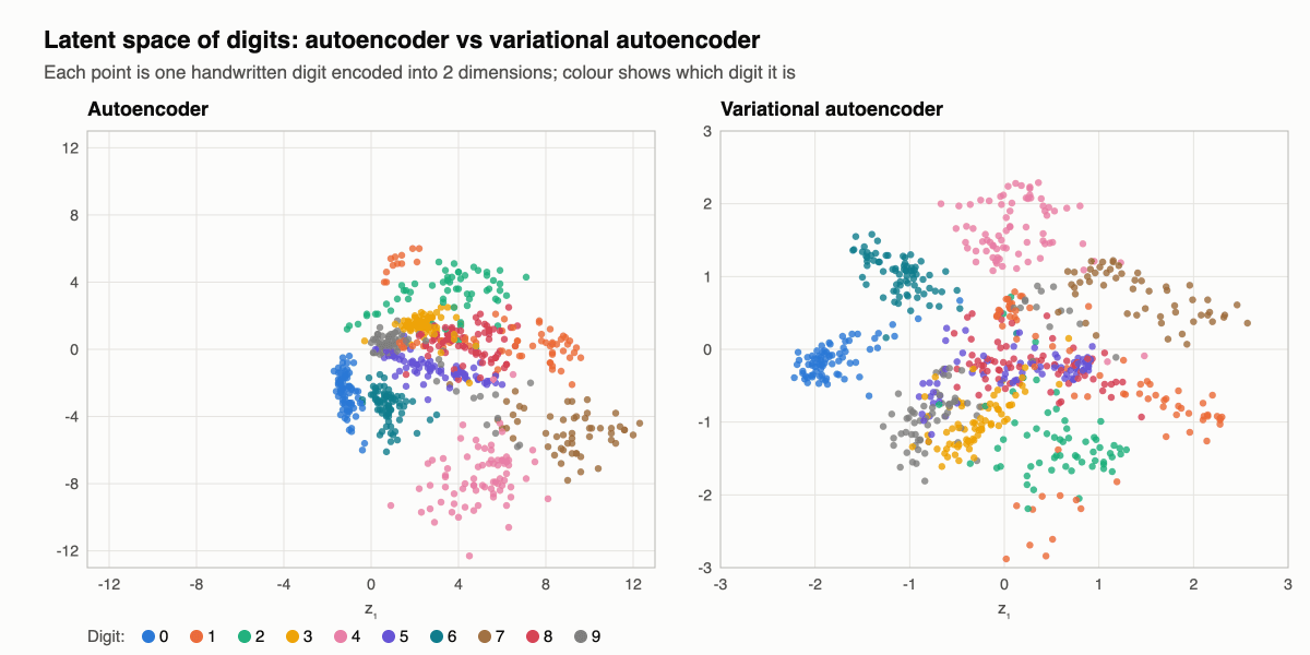
The autoencoder spreads its codes over a range from about −12 to 12, with an irregular shape and empty regions: there is no obvious way to choose a point that will decode into a valid digit. The VAE packs the same digits into a compact region around the origin, within about ±3 — close to a standard normal distribution — with the classes still separated but touching each other. Note the different axis scales of the two plots.
How a VAE Works
The VAE gets a continuous latent space by a surprising change: the encoder outputs not one vector of size n but two — a vector of means μ and a vector of standard deviations σ. Together they describe a normal distribution N(μ, σ²) for every input, and the code z that goes into the decoder is sampled from it:
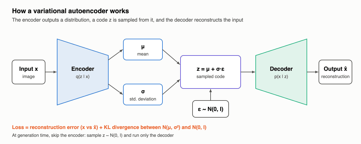
- The encoder maps the input
xtoμandσ. In probabilistic terms it approximates the posterior distributionq(z | x). - A latent vector
zis sampled fromN(μ, σ²). Because of the randomness, the same input produces a slightly different code every time. - The decoder maps
zback to a reconstructionx̂; it modelsp(x | z).
Sampling means that each input is represented not by a single point but by a small region of the latent space: the mean says where the region is centred, the standard deviation how wide it is. The decoder learns that every point in that region should decode into something close to the input, which makes the latent space locally continuous.
That alone is not enough. Nothing so far stops the encoder from placing the regions of different inputs far apart and making σ tiny, which would bring us back to a plain autoencoder with isolated points. This is what the second part of the loss prevents.
The VAE Loss: Reconstruction and KL Divergence
The VAE loss has two terms:
Loss = reconstruction loss + KL( N(μ, σ²) ‖ N(0, I) )
The reconstruction loss measures how well the output matches the input, as in an ordinary autoencoder: binary cross-entropy for images with pixel values between 0 and 1, mean squared error for real-valued data.
The Kullback–Leibler divergence (KL divergence) measures how different two probability distributions are. Here it compares each encoded distribution with the standard normal distribution N(0, I). For normal distributions it has a closed form, summed over the n latent dimensions:
KL = −½ · Σ (1 + log σᵢ² − μᵢ² − σᵢ²)
It is zero only when μ = 0 and σ = 1 in every dimension. The KL term penalizes the encoder for moving codes far from the origin and for making the distributions too narrow, so the regions of all inputs are pulled together around the origin and overlap.
The two terms pull in opposite directions. With the KL term alone, every input would be encoded as the same N(0, I) and the decoder could not tell them apart. With the reconstruction term alone, we get a plain autoencoder. Optimizing both gives a compromise: similar inputs end up close together, different inputs stay distinguishable, and the whole latent space is densely packed around the origin without gaps — exactly the VAE plot above.
The evidence lower bound (ELBO)
The loss is not an ad hoc combination. A VAE is trained to maximize the likelihood of the data, log p(x), which cannot be computed directly. Variational inference gives a lower bound on it, the evidence lower bound:
log p(x) ≥ Eq(z|x)[ log p(x | z) ] − KL( q(z | x) ‖ p(z) )
The first term is the expected reconstruction quality, the second is the KL divergence from the prior p(z) = N(0, I). Maximizing the ELBO is the same as minimizing the VAE loss above, so training a VAE is approximate maximum likelihood.
The Reparameterization Trick
There is a technical problem: backpropagation cannot pass through a random sampling step. If z is simply drawn from N(μ, σ²), there is no gradient of z with respect to μ and σ, and the encoder cannot learn.
The reparameterization trick moves the randomness out of the way. Sample noise ε from a fixed standard normal distribution and compute
z = μ + σ · ε, ε ~ N(0, I)
The result has exactly the same distribution, but now z is a deterministic, differentiable function of μ and σ, with all the randomness in an input ε that needs no gradient. The gradients flow through μ and σ to the encoder as usual. In practice the encoder outputs log σ² rather than σ, which keeps the standard deviation positive and the training numerically stable.
Exploring the Latent Space
Because every point of a trained VAE latent space decodes into something plausible, we can walk through it. Below, our two-dimensional VAE decodes a regular grid of 225 points between −2.5 and 2.5 in both dimensions. None of these images exist in the dataset; each is generated by the decoder:
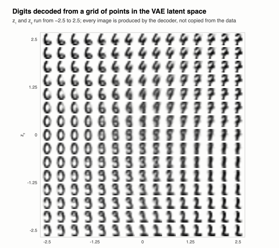
The digits change gradually from one cell to the next, and one digit morphs smoothly into another — for example 6 into 0 on the left. This smooth structure enables three useful operations:
- Sampling. To generate a new example, draw
zfromN(0, I)and decode it. Thanks to the KL term, this is exactly where the training data lives. - Interpolation. To create something halfway between two examples, encode both, take the midpoint of their mean vectors and decode it. Moving along the line between the two codes produces a smooth transition.
- Latent arithmetic. To add a feature, such as glasses on a portrait, encode similar images with and without glasses, take the difference of their codes, and add this “glasses vector” to the code of any other face before decoding.
Variational Autoencoder in PyTorch
The complete VAE below is trained on the handwritten digits dataset that ships with scikit-learn, so it runs in a minute or two on a CPU without downloading anything. The encoder and decoder are small fully connected networks with a two-dimensional latent space, the same model as in the figures above:
import torch
import torch.nn as nn
import torch.nn.functional as F
from sklearn.datasets import load_digits

torch.manual_seed(0)
digits = load_digits()
X = torch.tensor(digits.data, dtype=torch.float32) / 16.0     # 1,797 images, 64 pixels in [0, 1]

class VAE(nn.Module):
    def __init__(self, n_in=64, n_hidden=128, n_latent=2):
        super().__init__()
        self.encoder = nn.Sequential(nn.Linear(n_in, n_hidden), nn.ReLU())
        self.to_mu = nn.Linear(n_hidden, n_latent)              # mean of q(z|x)
        self.to_logvar = nn.Linear(n_hidden, n_latent)          # log variance of q(z|x)
        self.decoder = nn.Sequential(nn.Linear(n_latent, n_hidden), nn.ReLU(),
                                     nn.Linear(n_hidden, n_in))  # logits of the pixels

    def forward(self, x):
        h = self.encoder(x)
        mu, logvar = self.to_mu(h), self.to_logvar(h)
        eps = torch.randn_like(mu)
        z = mu + torch.exp(0.5 * logvar) * eps                   # reparameterization trick
        return self.decoder(z), mu, logvar

def vae_loss(logits, x, mu, logvar):
    recon = F.binary_cross_entropy_with_logits(logits, x, reduction="sum")
    kl = -0.5 * torch.sum(1 + logvar - mu ** 2 - logvar.exp())   # KL(q(z|x) || N(0, I))
    return recon, kl

model = VAE()
opt = torch.optim.Adam(model.parameters(), lr=1e-3)
for epoch in range(1, 201):
    for i in torch.randperm(len(X)).split(64):
        logits, mu, logvar = model(X[i])
        recon, kl = vae_loss(logits, X[i], mu, logvar)
        loss = (recon + kl) / len(i)
        opt.zero_grad()
        loss.backward()
        opt.step()
    if epoch in (1, 50, 200):
        with torch.no_grad():
            logits, mu, logvar = model(X)
            recon, kl = vae_loss(logits, X, mu, logvar)
        print(f"epoch {epoch:3d}: reconstruction {recon / len(X):.1f}, KL {kl / len(X):.2f} per image")

# Generate new digits: sample z from the prior N(0, I) and decode
with torch.no_grad():
    z = torch.randn(8, 2)
    samples = torch.sigmoid(model.decoder(z)).reshape(8, 8, 8)
print("generated:", samples.shape)
Output:
epoch   1: reconstruction 31.5, KL 1.59 per image
epoch  50: reconstruction 22.8, KL 2.10 per image
epoch 200: reconstruction 22.0, KL 2.44 per image
generated: torch.Size([8, 8, 8])
The reconstruction loss falls during training while the KL term grows a little: the encoder learns to use the latent space to carry information about each digit, paying a small KL price for it. The last lines generate eight new digits by decoding random points from the prior. For real images, replace the fully connected layers with convolutional ones and use a larger latent space, typically 16 to 512 dimensions.
Checking the KL formula
The closed-form KL term in vae_loss is easy to get wrong. It can be verified against PyTorch’s own implementation and a Monte Carlo estimate:
import torch
from torch.distributions import Normal, kl_divergence

mu, sigma = torch.tensor(1.5), torch.tensor(0.5)
closed_form = -0.5 * (1 + torch.log(sigma ** 2) - mu ** 2 - sigma ** 2)
library = kl_divergence(Normal(mu, sigma), Normal(0.0, 1.0))
z = Normal(mu, sigma).sample((1_000_000,))
monte_carlo = (Normal(mu, sigma).log_prob(z) - Normal(0.0, 1.0).log_prob(z)).mean()
print(f"closed form {closed_form:.4f}, torch {library:.4f}, Monte Carlo {monte_carlo:.4f}")
Output:
closed form 1.4431, torch 1.4431, Monte Carlo 1.4433VAE Variants
| Variant | Year | Idea | Used for |
|---|---|---|---|
| Conditional VAE (CVAE) | 2015 | Encoder and decoder also receive a label, such as the digit class | Generating examples of a chosen class |
| β-VAE | 2017 | Multiplies the KL term by β > 1 to force a more structured latent space | Disentangled representations, where each dimension controls one factor such as pose or lighting |
| VQ-VAE | 2017 | Replaces the continuous latent space with a discrete codebook of learned vectors | Sharp images and audio; tokenizers for image and speech generation models |
| Hierarchical VAE (NVAE, VDVAE) | 2020 | Many layers of latent variables at different resolutions | High-quality image generation with a VAE |
| VAE in latent diffusion | 2022 | A KL-regularized autoencoder compresses images; a diffusion model generates in its latent space | Stable Diffusion and similar image generators |
The last row is where most people meet VAEs today. In Stable Diffusion, a VAE encoder compresses a 512×512 RGB image into a 64×64×4 latent, the diffusion model does all its work in this much smaller space, and the VAE decoder turns the result back into pixels. The VAE is what makes generating large images affordable.
VAEs also work beyond images. With recurrent or Transformer encoders and decoders they handle sequences: Google Magenta’s MusicVAE interpolates between melodies, and VAEs are used to generate text and molecules.
VAE vs GAN vs Diffusion Models
| VAE | GAN | Diffusion model | |
|---|---|---|---|
| How it learns | Encoder and decoder maximize a lower bound on the likelihood | A generator tries to fool a discriminator | A network learns to remove noise step by step |
| Training | Stable, one loss | Unstable, prone to mode collapse | Stable |
| Sample quality | Often blurry | Sharp | Sharp, highest diversity |
| Generation speed | One decoder pass | One generator pass | Many denoising steps |
| Encoder for existing data | Yes | No, needs extra work | Indirect |
| Latent space | Smooth and structured | Usable but no encoder | Same size as the data, or a VAE latent |
VAE samples are blurry because the decoder is trained to predict the average of all images that are plausible for a code, and averaging sharp details blurs them. GANs and diffusion models do not average in this way. In practice the approaches are often combined: VQ-VAE codes or VAE latents feed Transformers and diffusion models, and VAE-GAN hybrids add an adversarial loss to sharpen VAE outputs.
Applications and Limitations
Variational autoencoders are used for:
- image generation and editing, including the latent space of diffusion image generators;
- anomaly detection in manufacturing, finance and medicine: inputs with a high reconstruction error or a low likelihood are suspicious;
- representation learning, where the latent codes serve as compact features for other models;
- drug discovery, by generating and optimizing molecules in a continuous latent space;
- data augmentation and synthetic data, and music and speech generation.
The main limitations are the blurriness of samples, the balance between the two loss terms, which often needs tuning, and posterior collapse: with a very powerful decoder, such as an autoregressive one, the model may learn to ignore the latent code entirely, driving the KL term to zero. Common fixes are gradually increasing the weight of the KL term during training (KL annealing) and limiting the decoder.
FAQ
What is a variational autoencoder in simple terms?
It is a neural network that learns to compress data into a few numbers and to rebuild it, in such a way that any combination of those numbers produces realistic data. That makes it possible to generate new examples and smoothly blend existing ones.
What is the difference between an autoencoder and a variational autoencoder?
An autoencoder maps each input to a single point and only learns to reconstruct; its latent space can have gaps. A VAE maps each input to a probability distribution and adds a KL term to the loss, which makes the latent space continuous and suitable for generating new data.
Why is the KL divergence used in a VAE?
It keeps the distributions produced by the encoder close to a standard normal distribution. Without it the encoder could scatter the codes anywhere, and sampling from N(0, I) would not produce realistic outputs.
What is the reparameterization trick?
It rewrites sampling as z = μ + σ · ε, where ε is random noise from a standard normal distribution. This makes z a differentiable function of the encoder outputs, so the model can be trained with backpropagation.
Is Stable Diffusion a VAE?
No, but it contains one. Stable Diffusion is a latent diffusion model: a VAE compresses images into a smaller latent space, the diffusion model generates in that space, and the VAE decoder converts the result back into an image.
See also: our guides to backpropagation and gradient descent, which train the encoder and decoder of every VAE.