Data science interviews test a wide mix of skills: statistics and probability, machine learning, SQL and Python, experiment design, product thinking and communication. The questions differ by company and role, but the same core topics come up again and again, from “explain the bias-variance trade-off” to “write a query for the second-highest salary” and “how would you measure the success of a new feature?”
This guide collects the most common data science interview questions with short, interview-ready answers, grouped by topic. For the questions that have a precise answer, such as probability puzzles, A/B test sizing, SQL and pandas tasks, we wrote and ran Python code to check the answers; the script and its output are included. It also explains how the interview process works in 2026, including the new AI-assisted coding rounds, and how to prepare.
Key takeaways
- A typical loop has five parts: recruiter screen, technical screen (SQL or Python), a take-home or case study, an onsite or virtual loop of 4 to 6 interviews, and a behavioral round.
- The core topics are statistics and probability, A/B testing, machine learning fundamentals, SQL, Python and pandas, product sense and, for ML roles, system design. Questions on LLMs and retrieval-augmented generation have become common since 2024.
- AI is entering interviews. Meta began rolling out an AI-enabled coding round in October 2025, and Google is piloting an AI-assisted round with Gemini in 2026. Interviewers increasingly check how you verify and debug code, not only whether you can write it.
- Classic puzzles trip people up: the chance that a family with at least one boy has two boys is 1/3, not 1/2, and an A/B test that looks for a 2% lift on a 10% conversion rate needs about 356,000 users per group.
- The job market is growing: the US Bureau of Labor Statistics projects 35% employment growth for data scientists from 2025 to 2035, with a median wage of $120,230 in May 2025.
How data science interviews work in 2026
“Data scientist” covers several different jobs, and the interview follows the job. Product or analytics data scientists work on metrics, experiments and dashboards; their interviews stress SQL, statistics, A/B testing and product sense. Machine learning data scientists and ML engineers build and deploy models; they get more coding, ML theory and system design. Research scientists are asked about papers, deep learning and mathematics. Read the job description carefully: it tells you which questions to expect.
Most companies use a similar sequence of stages:
| Stage | What happens | What is tested |
|---|---|---|
| Recruiter screen | A 20 to 30 minute call about your background, motivation and expectations | Fit with the role, communication |
| Technical screen | A live coding session or an online test, often on a shared editor or a platform such as CodeSignal, HackerRank or Codility | SQL, Python, basic statistics |
| Take-home or case study | A data set with questions to answer in a few hours or days, or a business case discussed live | Analysis, modeling, judgment, presentation |
| Onsite or virtual loop | Four to six interviews of 45 to 60 minutes with different team members | Statistics, ML, experimentation, product sense, coding, system design |
| Behavioral round | Questions about past projects, conflicts and mistakes | Collaboration, ownership, communication with non-technical people |
Two changes stand out in 2026. First, AI tools are entering technical rounds. Meta began rolling out an AI-enabled coding interview in October 2025, in which candidates can use an AI assistant, and Google started piloting an “AI-assisted” coding round with its Gemini model for some engineering roles in 2026. In these rounds, interviewers look at how you break down the problem, check and debug the generated code and explain your choices. Many companies still forbid AI tools in other rounds, so ask the recruiter about the rules. Second, LLM questions are standard: even analytics roles are often asked how they would evaluate or apply a large language model.
The market remains strong. The US Bureau of Labor Statistics counted about 275,600 data scientist jobs in 2025, with a median wage of $120,230 in May 2025, and projects 35% employment growth from 2025 to 2035, about 24,800 openings per year.
Statistics and probability questions
1. What is a p-value?
The probability of seeing data at least as extreme as what was observed, if the null hypothesis were true. It is not the probability that the null hypothesis is true. A p-value below the chosen significance level, usually 0.05, means the result would be surprising under the null hypothesis, so we reject it.
2. What are type I and type II errors?
A type I error is a false positive: rejecting a true null hypothesis, for example shipping a feature that does not work. Its probability is the significance level α. A type II error is a false negative: missing a real effect. Its probability is β, and power, 1 − β, is the probability of detecting an effect that really exists.
3. Explain the central limit theorem.
The mean of many independent draws from almost any distribution with finite variance is approximately normally distributed, with standard deviation σ / √n, even if the original distribution is skewed. It is why confidence intervals and z-tests work for averages and conversion rates. In our code below, single draws from an exponential distribution have a skewness of 1.98, but means of just 30 draws have a skewness of 0.37 and a standard deviation of 0.182, matching the theoretical 1/√30 = 0.183.
4. What is the difference between a confidence interval and a credible interval?
A 95% confidence interval is a frequentist statement about the procedure: if we repeated the experiment many times, 95% of the intervals would contain the true value. A 95% credible interval is Bayesian: given the data and the prior, there is a 95% probability that the parameter lies in the interval. See our guide to Bayes’ theorem for the Bayesian view.
5. A family has two children, and at least one is a boy. What is the probability that both are boys?
1/3. The equally likely families are boy-boy, boy-girl, girl-boy and girl-girl; knowing that at least one is a boy removes girl-girl, and only one of the three remaining cases has two boys. The intuitive answer, 1/2, is the answer to a different question: “the older child is a boy”. Our simulation of a million families gives 0.3332.
6. Which is more likely: at least one six in 6 rolls of a die, at least two sixes in 12 rolls, or at least three in 18?
At least one six in 6 rolls: 66.5%, against 61.9% for two in 12 and 59.7% for three in 18. This is the Newton–Pepys problem, which Samuel Pepys asked Isaac Newton in 1693. The expected number of sixes is the same, one per six rolls, but the chance of reaching at least that number falls as the number of rolls grows, towards 50%: for at least 100 sixes in 600 rolls it is 51.7%. Compute it with the binomial distribution: P(at least k) = 1 − Σi<k C(n, i) (1/6)i (5/6)n−i.
7. A test for a disease is 99% accurate and 1% of people have the disease. You test positive. How likely are you to be sick?
About 50%. Out of 10,000 people, 100 are sick and 99 of them test positive; of the 9,900 healthy people, 1% or 99 also test positive. So half of the 198 positives are sick. This is Bayes’ theorem in action, and the lesson is to always consider the base rate.
8. What is the difference between correlation and causation? Give an example of a confounder.
Correlation measures how two variables move together; causation means changing one changes the other. Ice cream sales and drownings are correlated because both rise in summer: temperature is a confounder that causes both. Randomized experiments break confounding; with observational data, use methods such as matching, difference-in-differences or instrumental variables, and state assumptions clearly.
9. What is Simpson’s paradox?
A trend that appears in every subgroup can reverse when the groups are combined, because the groups have different sizes or mixes. A classic case: a treatment can have a higher success rate than another for both small and large kidney stones, yet a lower success rate overall, because it was used more often on the harder, large stones. Always check whether an aggregate result holds within important segments.
10. When would you use the median instead of the mean?
When the data is skewed or has outliers, such as income, house prices, session lengths or delivery times. A few extreme values pull the mean far away, while the median describes the typical case. Report both, or a few percentiles, when the distribution matters.
A/B testing and experimentation questions
11. How do you design an A/B test?
Define the hypothesis and one primary metric, plus guardrail metrics that must not get worse (such as latency or unsubscribes). Choose the unit of randomization, usually the user. Fix the significance level, power and the minimum detectable effect, compute the sample size, decide the duration in advance (at least one or two full weeks to cover weekly cycles), run the test, check data quality, and only then analyse the result.
12. How many users do you need?
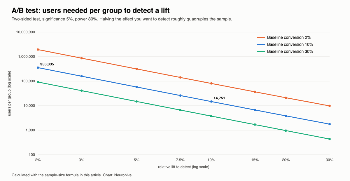
For conversion rates, the sample size per group is roughly n ≈ (z1−α/2 + z1−β)² × [p1(1 − p1) + p2(1 − p2)] / (p1 − p2)². The key insight is that it grows with the inverse square of the effect: in our calculation for a 10% baseline conversion rate, detecting a 20% relative lift needs 3,841 users per group, a 10% lift 14,751, a 5% lift 57,763 and a 2% lift 356,335.
13. A test with 10,000 users per group shows 1,000 vs 1,080 conversions. Is the difference significant?
Not at the 5% level. A two-proportion z-test gives z = 1.85 and a two-sided p-value of 0.064. The observed lift of 8% is plausible, but the test was too small to detect it reliably: as the chart above shows, a 10% lift already needs almost 15,000 users per group. The right conclusion is “inconclusive”, not “no effect”.
14. What is wrong with checking results every day and stopping when p < 0.05?
This is peeking. Each look is another chance for a false positive, so the real false-positive rate can rise far above 5%. Either fix the sample size in advance and look once, or use methods designed for continuous monitoring, such as sequential tests or always-valid p-values.
15. You test 20 metrics and one is significant. What do you conclude?
Probably nothing. With 20 independent tests at α = 0.05, you expect one false positive by chance. Correct for multiple comparisons, for example with the Bonferroni correction (α / 20) or by controlling the false discovery rate, and decide on one primary metric before the test.
16. The split was meant to be 50/50, but the groups have 50,600 and 49,400 users. Is that a problem?
Probably yes: this is a sample ratio mismatch. A chi-square test on the counts gives χ² = 14.4 and a p-value of 0.00015, so the difference is unlikely to be chance. It usually signals a bug in assignment or logging, such as a redirect that loses users in one group, and invalidates the comparison until the cause is found.
17. When can you not run an A/B test, and what do you do instead?
When users influence each other (marketplaces, social networks), when the change cannot be shown to only part of the users (pricing, brand changes), or when it is unethical. Alternatives include cluster or geographic randomization, switchback tests that alternate treatment over time, and observational methods such as difference-in-differences or synthetic control. Watch also for novelty effects, where users react to change itself and the effect fades after a few weeks.
Machine learning interview questions
18. Explain the bias-variance trade-off.
Prediction error has three parts: bias, from wrong assumptions that make the model too simple (underfitting); variance, from sensitivity to the particular training data that makes the model too complex (overfitting); and irreducible noise. Making a model more flexible lowers bias but raises variance. Regularization, more data and ensembles help find the balance.
19. How do you detect and prevent overfitting?
Overfitting shows as a large gap between training and validation performance. Prevent it with cross-validation, simpler models, regularization (L1, L2, dropout), early stopping, more training data or data augmentation, and by removing leaked features.
20. What is the difference between L1 and L2 regularization?
Both add a penalty on the size of the weights to the loss. L1 (lasso) adds the sum of absolute values and pushes many weights to exactly zero, so it also selects features. L2 (ridge) adds the sum of squares and shrinks all weights smoothly, which handles correlated features better. Elastic net combines both.
21. How does logistic regression work?
It computes a weighted sum of the features, like linear regression, and passes it through the sigmoid function to get a probability between 0 and 1. It is trained by minimizing the log loss (cross-entropy), usually with gradient descent. Each coefficient is the change in the log-odds per unit change of a feature, which makes the model easy to interpret.
22. Explain precision, recall, F1 and ROC AUC. Which would you use for fraud detection?
Precision is the share of predicted positives that are real; recall is the share of real positives that the model finds; F1 is their harmonic mean. ROC AUC is the probability that a random positive gets a higher score than a random negative, independent of the threshold. For fraud, where positives are rare, accuracy is useless (99.9% by predicting “no fraud”), and ROC AUC can look good even when precision is poor; use precision-recall curves, PR AUC and the business cost of each error to choose a threshold.
23. How do you handle an imbalanced data set?
Use metrics that reflect the rare class (recall, precision, PR AUC), stratified splits, class weights in the loss, resampling (undersampling the majority or oversampling the minority, carefully, only on the training data), and threshold tuning. Often the best fix is more examples of the rare class.
24. How would you handle missing values?
First ask why they are missing: at random, or for a reason that is itself informative? Then choose: drop rows or columns with few useful values, impute with the median or the most frequent value, impute with a model, or let a model handle missing values natively, as gradient-boosted trees do. Adding an “is missing” indicator often helps, and imputation must be fitted on the training data only.
25. What is data leakage? Give an example.
Leakage happens when the model uses information that will not be available at prediction time, which makes validation scores look much better than real performance. Examples: a “cancellation date” column in a churn model, scaling or imputing on the whole data set before splitting, or random splits of time series, where the model effectively sees the future.
26. Explain cross-validation. When is a random split wrong?
In k-fold cross-validation, the data is split into k parts; each part serves once as the validation set while the model trains on the rest, and the k scores are averaged. A random split is wrong for time series (use forward-chaining splits that train on the past and test on the future) and for grouped data such as several rows per user or patient (use group splits so the same user is never in both training and validation).
27. How does a decision tree decide where to split?
It tries candidate splits of each feature and picks the one that most reduces impurity, measured by Gini impurity or entropy for classification and by variance for regression, then repeats recursively. Our decision tree guide walks through the algorithm with code.
28. What is the difference between bagging and boosting? Random forest vs gradient boosting?
Bagging trains many models independently on bootstrap samples and averages them, which reduces variance; random forest is bagging of deep trees with random feature subsets at each split. Boosting trains shallow models sequentially, each correcting the errors of the previous ones, which reduces bias. Gradient boosting (XGBoost, LightGBM, CatBoost) is usually the most accurate choice for tabular data but needs more tuning; random forests are robust with default settings.
29. How does k-means work, and how do you choose k?
Pick k initial centers, assign every point to its nearest center, move each center to the mean of its points, and repeat until assignments stop changing. Choose k with the elbow method (where the within-cluster variance stops dropping quickly), the silhouette score, or, best, by what makes sense for the business use. K-means assumes roughly spherical clusters of similar size and needs scaled features. It is an example of unsupervised learning.
30. What is PCA, and when would you use it?
Principal component analysis finds the orthogonal directions of maximum variance and projects the data onto the first few. It is used to compress correlated features, speed up models, remove noise and visualize high-dimensional data. The components are linear combinations of the original features, which makes them harder to interpret, and the features must be standardized first.
Deep learning and LLM questions
31. How does backpropagation work?
The network computes a prediction in a forward pass, measures the loss, and then applies the chain rule backward through the layers to compute the gradient of the loss with respect to every weight; an optimizer then updates the weights. Our guides to backpropagation and how neural networks work show it step by step.
32. What are vanishing and exploding gradients, and how do you fix them?
In deep networks, gradients are products of many terms; if those terms are mostly below 1, the gradients shrink to almost zero in the early layers, which stop learning; if above 1, they explode. Fixes: ReLU-family activation functions instead of sigmoid, careful weight initialization, normalization layers, residual connections, gradient clipping, and gated architectures such as LSTM for sequences.
33. Why do convolutional networks work well for images?
Convolutions share the same small filters across the whole image, so a pattern learned in one place is recognized anywhere, with far fewer parameters than a fully connected layer; stacking layers builds features from edges to textures to objects. See our CNN guide.
34. Explain self-attention in transformers.
Every token is turned into a query, a key and a value vector. The attention weights of a token are the softmax of the dot products of its query with all keys, divided by √d, and its output is the weighted sum of the values: softmax(QKᵀ / √d) V. This lets every token draw information directly from every other token, which made transformers better than recurrent networks at long-range dependencies and much easier to parallelize. Multi-head attention runs several such attention operations in parallel.
35. What are embeddings?
Dense vectors that represent items such as words, products or users so that similar items are close together. They are learned from data, from word2vec to the embedding layers of transformers, and are used for search, recommendations, clustering and as features for other models.
36. What is retrieval-augmented generation (RAG), and when would you use it instead of fine-tuning?
RAG retrieves relevant documents, usually with embedding search over a vector index, and adds them to the prompt so that the LLM answers from up-to-date, specific sources and can cite them. Use RAG when the model needs knowledge that changes or is private; use fine-tuning when it needs a new behavior, style or format. Prompting is the cheapest first step, and the approaches are often combined.
37. How would you evaluate an LLM application?
Build a test set of realistic inputs with reference answers or grading rules. Measure task success with automatic checks where possible (exact match, unit tests, structured-output validation), use LLM-as-a-judge with clear rubrics for open-ended answers and check it against human ratings, and track groundedness and hallucination rate for RAG, plus latency and cost. Online, monitor user feedback and A/B test changes.
38. Why do LLMs hallucinate, and how can you reduce it?
They generate the most plausible continuation of the text, not verified facts, so they can produce fluent but false statements, especially about rare facts. Reduce it with retrieval from trusted sources and instructions to answer only from them, citations, lower temperature, asking the model to say when it does not know, verification steps and human review for high-stakes outputs.
SQL interview questions
SQL questions test joins, aggregation and, above all, window functions. The answers below were run in SQLite; the code is in the code section.
39. Find the second-highest salary in each department.
Rank salaries within each department with a window function and keep rank 2. Use DENSE_RANK, not ROW_NUMBER, so that ties are handled: in the ML team with salaries 180, 150 and 150, the second-highest salary is 150.
SELECT dept, salary AS second_highest FROM (
    SELECT dept, salary, DENSE_RANK() OVER (PARTITION BY dept ORDER BY salary DESC) AS rnk
    FROM employees)
WHERE rnk = 2
GROUP BY dept;
40. Compute a 7-day rolling average of daily revenue.
SELECT day, revenue,
       AVG(revenue) OVER (ORDER BY day ROWS BETWEEN 6 PRECEDING AND CURRENT ROW) AS avg_7d
FROM sales;
Follow-up: if some days have no sales, the rows are missing and “6 preceding rows” is no longer 7 days. Join to a calendar table first, or use a RANGE window on dates where the database supports it.
41. What is the difference between WHERE and HAVING? Between INNER and LEFT JOIN?
WHERE filters rows before aggregation, HAVING filters groups after it. An INNER JOIN keeps only rows with a match in both tables; a LEFT JOIN keeps all rows of the left table and fills missing matches with NULL. A common trap is a WHERE condition on the right table that silently turns a left join into an inner join.
42. How do you find users who signed up but never made a purchase?
Left-join purchases to users and keep rows where the purchase is NULL, or use NOT EXISTS: SELECT u.id FROM users u WHERE NOT EXISTS (SELECT 1 FROM purchases p WHERE p.user_id = u.id). Avoid NOT IN with a subquery that can return NULL, which returns no rows at all.
43. How would you remove duplicate rows but keep the latest one per user?
Number the rows per user by time with ROW_NUMBER() OVER (PARTITION BY user_id ORDER BY updated_at DESC) and keep row 1.
Python and pandas questions
44. Compute 7-day retention for a cohort of users.
Find each user’s first active day, keep the cohort that started on a given day, and count how many were active again within the next 7 days. In our small example, 2 of the 4 users who started on 1 October came back within a week. The pandas code is in the code section.
45. How would you count the frequency of each number in a file too large to fit in memory?
Stream it: read line by line or in chunks (for example with pandas.read_csv(..., chunksize=...)) and update a collections.Counter, which needs memory only for the distinct values. If even those do not fit, hash values into buckets written to separate files and count each bucket, or use a tool built for out-of-core data such as DuckDB, Polars or Spark.
46. What is the difference between a list and a NumPy array? Why is vectorized code faster?
A list holds references to arbitrary Python objects; a NumPy array holds numbers of one type in a contiguous block of memory. Vectorized operations run in compiled code over the whole block instead of executing a Python loop step for each element, which is typically 10 to 100 times faster.
47. What do groupby().transform() and merge() do in pandas?
transform returns a result with the same shape as the input, aligned to the original rows, for example each user’s first day next to every event of that user; agg instead returns one row per group. merge joins two data frames on keys like a SQL join, with how="inner", "left", "right" or "outer"; check row counts after merging to catch unintended many-to-many joins.
The answers in code
This script checks the answers to questions 3, 5, 6, 12, 13, 16, 39, 40 and 44 by simulation and direct computation. It needs NumPy, pandas and SciPy and runs in a few seconds:
import sqlite3
from math import comb

import numpy as np
import pandas as pd
from scipy import stats

rng = np.random.default_rng(0)
N = 1_000_000

# 1. Probability: a family has two children, at least one is a boy. Probability both are boys?
kids = rng.integers(0, 2, size=(N, 2))                      # 1 = boy
at_least_one_boy = kids.max(1) == 1
print(f"Two boys | at least one boy: simulated {kids[at_least_one_boy].min(1).mean():.4f}, exact {1/3:.4f}")

# 2. Probability: which is likelier, at least one six in 6 rolls, two in 12 or three in 18? (Newton-Pepys problem)
def p_at_least(k, n):                                       # P(at least k sixes in n rolls), exact
    return 1 - sum(comb(n, i) * (1 / 6) ** i * (5 / 6) ** (n - i) for i in range(k))
for k, n in [(1, 6), (2, 12), (3, 18), (100, 600)]:
    sim = (rng.integers(1, 7, size=(200_000, n)) == 6).sum(1) >= k
    print(f"At least {k:3d} six(es) in {n:3d} rolls: exact {p_at_least(k, n):.4f}, simulated {sim.mean():.4f}")

# 3. Statistics: why does the sample mean become normal? Central limit theorem on a skewed distribution
skewed = rng.exponential(1.0, size=(100_000, 30))           # skewness of a single draw = 2
means = skewed.mean(1)
print(f"Exponential draws: skewness {stats.skew(skewed[:, 0]):.2f}; means of 30 draws: skewness {stats.skew(means):.2f}, "
      f"std {means.std():.3f} (theory {1 / np.sqrt(30):.3f})")

# 4. A/B testing: sample size per group to detect a lift in conversion from 10% (alpha 0.05, power 0.8)
def sample_size(p1, p2, alpha=0.05, power=0.8):
    z_a, z_b = stats.norm.ppf(1 - alpha / 2), stats.norm.ppf(power)
    p_bar = (p1 + p2) / 2
    return int(np.ceil((z_a * np.sqrt(2 * p_bar * (1 - p_bar)) + z_b * np.sqrt(p1 * (1 - p1) + p2 * (1 - p2))) ** 2
                       / (p1 - p2) ** 2))
for lift in [0.20, 0.10, 0.05, 0.02]:
    print(f"Baseline 10%, relative lift {lift:4.0%}: {sample_size(0.10, 0.10 * (1 + lift)):>9,} users per group")

# A finished test: 10,000 users per group, 1,000 vs 1,080 conversions. Is the difference significant?
conv, n = np.array([1000, 1080]), np.array([10_000, 10_000])
p_pool = conv.sum() / n.sum()
z = (conv[1] / n[1] - conv[0] / n[0]) / np.sqrt(p_pool * (1 - p_pool) * (1 / n[0] + 1 / n[1]))
print(f"Two-proportion z-test: z = {z:.2f}, p-value = {2 * stats.norm.sf(abs(z)):.3f}")

# Sample ratio mismatch: a 50/50 split produced 50,600 and 49,400 users
chi2, p_srm = stats.chisquare([50_600, 49_400])
print(f"Sample ratio mismatch check: chi-square = {chi2:.1f}, p-value = {p_srm:.5f}")

# 5. SQL: second-highest salary per department, and 7-day rolling average of daily revenue
db = sqlite3.connect(":memory:")
pd.DataFrame({"name": ["Ann", "Bob", "Cid", "Dee", "Eva", "Fay"],
              "dept": ["ML", "ML", "ML", "BI", "BI", "BI"],
              "salary": [180, 150, 150, 120, 140, 110]}).to_sql("employees", db, index=False)
print(pd.read_sql("""
    SELECT dept, salary AS second_highest FROM (
        SELECT dept, salary, DENSE_RANK() OVER (PARTITION BY dept ORDER BY salary DESC) AS rnk FROM employees)
    WHERE rnk = 2 GROUP BY dept""", db).to_string(index=False))

days = pd.date_range("2026-10-01", periods=10).strftime("%Y-%m-%d")
pd.DataFrame({"day": days, "revenue": [100, 120, 90, 110, 130, 150, 140, 160, 120, 170]}).to_sql("sales", db, index=False)
print(pd.read_sql("""
    SELECT day, revenue, ROUND(AVG(revenue) OVER (ORDER BY day ROWS BETWEEN 6 PRECEDING AND CURRENT ROW), 1) AS avg_7d
    FROM sales""", db).tail(3).to_string(index=False))

# 6. pandas: users active on day 1 who came back within 7 days (retention)
events = pd.DataFrame({"user": [1, 1, 2, 3, 3, 4, 4, 5],
                       "day": pd.to_datetime(["2026-10-01", "2026-10-05", "2026-10-01", "2026-10-01", "2026-10-12",
                                              "2026-10-01", "2026-10-02", "2026-10-03"])})
first = events.groupby("user").day.transform("min")
cohort = events[first == "2026-10-01"]
returned = cohort[(cohort.day > first[cohort.index]) & (cohort.day <= first[cohort.index] + pd.Timedelta(days=7))]
print(f"7-day retention of the 2026-10-01 cohort: {returned.user.nunique()} of {cohort.user.nunique()} users")
Two boys | at least one boy: simulated 0.3332, exact 0.3333
At least 1 six(es) in 6 rolls: exact 0.6651, simulated 0.6646
At least 2 six(es) in 12 rolls: exact 0.6187, simulated 0.6177
At least 3 six(es) in 18 rolls: exact 0.5973, simulated 0.5972
At least 100 six(es) in 600 rolls: exact 0.5170, simulated 0.5154
Exponential draws: skewness 1.98; means of 30 draws: skewness 0.37, std 0.182 (theory 0.183)
Baseline 10%, relative lift 20%: 3,841 users per group
Baseline 10%, relative lift 10%: 14,751 users per group
Baseline 10%, relative lift 5%: 57,763 users per group
Baseline 10%, relative lift 2%: 356,335 users per group
Two-proportion z-test: z = 1.85, p-value = 0.064
Sample ratio mismatch check: chi-square = 14.4, p-value = 0.00015
dept second_highest
BI 120
ML 150
day revenue avg_7d
2026-10-08 160 128.6
2026-10-09 120 128.6
2026-10-10 170 140.0
7-day retention of the 2026-10-01 cohort: 2 of 4 usersProduct sense and case study questions
Product questions have no single right answer. Interviewers look for structure: clarify the goal, define metrics, consider trade-offs and segments, and propose how to measure.
48. A home-rental marketplace launches in a new city. How do you measure success?
Start with the goal: liquidity of a two-sided marketplace. Supply metrics: active listings, share of listings with bookings, host retention. Demand metrics: searches, booking conversion, nights booked, repeat guests. Balance: search-to-booking rate and share of searches with no available results. Quality and guardrails: cancellation rate, reviews, support tickets. Compare against similar past launches, not just against zero.
49. Daily active users dropped 10% yesterday. How do you investigate?
First check that the data is right (logging changes, pipeline delays, a time-zone shift). Then check whether it is external (holidays, outages, a competitor launch, seasonality compared with the same day last week). Then segment: platform, app version, country, new vs returning users, traffic source. A drop concentrated in one segment, such as a new Android version, usually points to the cause.
50. How would you build a model to detect fraudulent transactions?
Clarify the cost of each error: a missed fraud vs a blocked honest customer. Features: transaction amount relative to the user’s history, velocity (transactions per hour), device and IP changes, distance between locations, merchant risk, account age. Use time-based splits, handle extreme imbalance, choose the threshold by expected cost, and plan for delayed labels (chargebacks arrive weeks later) and fraudsters adapting to the model. Gradient boosting is a strong baseline; graph features help detect fraud rings.
51. You have two years of transaction history. Which features would you use to predict credit risk?
Income stability and its trend, debt-to-income ratio, credit utilization, payment history and missed payments, cash-flow volatility, spending categories, overdrafts and account tenure, all computed only from data available before the prediction date. Mention fairness and regulation: in lending, models must be explainable, and features that act as proxies for protected characteristics must be avoided.
52. How would you explain a statistical result to a non-technical stakeholder?
Lead with the decision and the business impact, give the uncertainty in plain words (“we are fairly confident the change adds between 1% and 4% to bookings”), use one clear chart, and keep methodology for questions. Avoid “p-value” and “statistically significant” unless the audience uses them.
ML system design questions
For ML roles, system design rounds ask you to design an end-to-end system: design a recommendation feed, a search ranking system, a spam filter, an ETA prediction service. A good answer covers:
- Problem and metrics. The business goal, the ML objective, offline metrics (such as NDCG for ranking) and online metrics measured in A/B tests.
- Data and labels. Where labels come from (clicks, purchases, human ratings), their biases, and how to avoid leakage.
- Features and model. Start with a simple baseline, then a stronger model; for recommendations, a fast candidate-generation stage (such as embedding retrieval) followed by a heavier ranking model.
- Serving. Latency budget, batch vs real-time features, caching, scaling.
- Monitoring and iteration. Data and prediction drift, retraining schedule, feedback loops, fallback behavior when the model fails.
53. How do you know when a deployed model needs retraining?
Monitor input data distributions, prediction distributions and, when labels arrive, model performance; alert on significant drift or drops. Many teams also retrain on a fixed schedule and compare the new model with the current one on recent data before switching.
54. Your offline metric improved, but the A/B test shows no gain. Why?
The offline metric may not reflect user value, the offline data may be biased by the old model’s choices (users only clicked what they were shown), there may be leakage in offline evaluation, latency may have increased, or the effect may be too small for the test to detect.
55. How would you make a model’s predictions explainable?
Use an interpretable model where possible (linear models, small trees); for complex models, show global feature importance and local explanations such as SHAP values for individual predictions, and validate explanations with domain experts. In regulated areas such as lending, explanations are a legal requirement.
Behavioral questions
Answer with the STAR structure: situation, task, action, result, ideally with a number in the result. Prepare four or five stories that you can adapt.
- 56. Tell me about a project you are proud of. Pick one with a measurable impact and explain your own role and decisions.
- 57. Tell me about a time your analysis was wrong or a model failed. Show that you found the cause, fixed it and changed your process.
- 58. Tell me about a disagreement with a stakeholder. Show that you listened, used data and reached a decision, even if it was not yours.
- 59. How do you prioritize when several teams ask for analysis? Talk about impact, effort, deadlines and making trade-offs explicit.
- 60. Why this company? Connect your experience with their product, data and problems; mention something specific you learned about them.
How to prepare
- Know the role. Analytics roles: SQL, statistics, experiments and product cases. ML roles: coding, ML theory and system design. Research roles: papers and deep learning.
- Practise SQL and Python daily for a few weeks, with an emphasis on window functions, joins, groupby and edge cases such as NULLs and ties.
- Review fundamentals: probability, hypothesis testing, the algorithms above and when to use them. Our guides to artificial intelligence and deep learning are a good refresher.
- Build or polish one end-to-end project that you can discuss in depth: the data, the choices, what went wrong and the result. A well-documented Kaggle project such as our Titanic tutorial is a good start, but a project on real, messy data stands out more.
- Practise explaining out loud, with mock interviews if possible. Thinking aloud, asking clarifying questions and stating assumptions matter as much as the final answer.
- Prepare for AI-assisted rounds: practise solving problems with an AI assistant, then reading, testing and fixing its code critically, and explain why you accept or reject its suggestions.
FAQ
What are the most common data science interview questions?
Explaining the bias-variance trade-off and overfitting, precision vs recall, how to handle missing values and imbalanced data, designing and analysing an A/B test, p-values, SQL queries with joins and window functions, a pandas data manipulation task, a product metric case, and “tell me about a project you worked on”.
How hard are data science interviews?
They are broad rather than extremely deep: you need solid basics in several areas at once. Most candidates find the combination of live coding, statistics and open-ended product questions the hardest part, which is why practising out loud matters.
Do data scientists need LeetCode?
For analytics and product data science roles, usually only easy to medium problems, mostly SQL and data manipulation in Python. ML engineering roles at large tech companies may include standard algorithm questions similar to software engineering interviews.
What is the difference between a data analyst and a data scientist interview?
Data analyst interviews focus on SQL, spreadsheets, dashboards, descriptive statistics and business questions. Data scientist interviews add statistical inference, experimentation, machine learning and often more coding.
How long does a data science interview process take?
Usually three to six weeks from the first call to the offer, with four to eight hours of interviews in total, plus a take-home assignment at some companies.