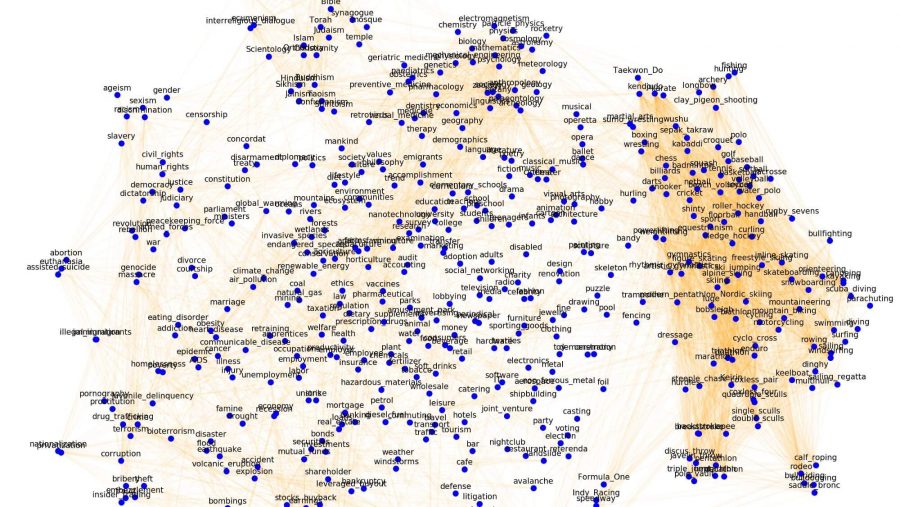
Word2vec is a method for turning words into vectors, lists of numbers, so that words with similar meanings get similar vectors. It was published by Tomas Mikolov and colleagues at Google in 2013 and quickly became one of the most influential ideas in natural language processing (NLP): it showed that a very simple neural network trained on raw text learns meaning well enough to solve analogies such as king − man + woman ≈ queen. Today’s large language models, semantic search and RAG systems all rely on embeddings, the idea that word2vec made popular.
This guide explains what word2vec is, how word embeddings work, the two word2vec architectures (CBOW and skip-gram), the training tricks that make it fast (negative sampling and subsampling), and how word2vec compares with GloVe, fastText and modern contextual embeddings such as BERT. We trained word2vec ourselves on 17 million words of Wikipedia: once from scratch in PyTorch to show every step, and once with the gensim library to compare CBOW, skip-gram and pretrained GloVe vectors on Google’s analogy test.
Key takeaways
- Word2vec learns a dense vector for every word by training a shallow neural network to predict words from their neighbours. Words that appear in similar contexts end up close together.
- Two architectures: CBOW predicts a word from its context and is faster; skip-gram predicts the context from a word and works better for rare words and semantic relations.
- Negative sampling replaces an expensive softmax over the whole vocabulary with a few binary “real or random pair?” decisions, which makes training on billions of words possible.
- In our experiment on 17 million words of Wikipedia, skip-gram solved 37.4% of Google’s analogy questions and CBOW 30.7%, while CBOW trained three times faster. Pretrained GloVe vectors, trained on 6 billion words, solved 65.5%: more data matters more than the choice of algorithm.
- Limitation: one vector per word, so “bank” (river) and “bank” (money) share a vector. Contextual models such as BERT and modern LLMs solve this, but word2vec remains a fast, cheap baseline.
What is word2vec?
Word2vec (“word to vector”) is a family of algorithms that learn word embeddings: a vector of typically 100 to 300 numbers for every word in a vocabulary. It was introduced in two 2013 papers by Tomas Mikolov, Kai Chen, Greg Corrado, Jeffrey Dean and Ilya Sutskever at Google. The second paper, “Distributed Representations of Words and Phrases and their Compositionality”, received the Test of Time Award at the NeurIPS conference in 2023, ten years after publication.
Before word2vec, most NLP systems represented words as one-hot vectors: a vector as long as the vocabulary, with a 1 in the position of the word and 0 everywhere else. One-hot vectors are huge, and they say nothing about meaning: “cat” is exactly as different from “dog” as from “pencil”. Word2vec replaces them with short, dense vectors learned from text, in which distance reflects similarity of meaning.
Google released the word2vec code together with vectors for 3 million words and phrases trained on about 100 billion words of Google News. Training was fast because the model is deliberately simple: no hidden layers with non-linear activations, just two tables of vectors and a clever training objective.
Word embeddings: meaning from context
Word2vec is built on the distributional hypothesis from linguistics, often summarised by J. R. Firth’s 1957 phrase “you shall know a word by the company it keeps”. Words that appear in similar contexts tend to have similar meanings. Consider the blanks below:
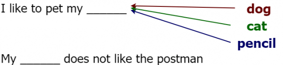
“Dog” and “cat” fit naturally; “pencil” does not. Nothing about spelling or grammar tells us this, only the contexts in which the words usually appear. Word2vec turns this observation into a training task: it learns vectors that are good at predicting which words appear near which. As a side effect, words with similar contexts receive similar vectors.
Similarity between two word vectors is usually measured with cosine similarity, the cosine of the angle between them: 1 means they point in the same direction, 0 means they are unrelated. The vectors also capture relations as directions. The difference between “paris” and “france” is roughly the same as between “berlin” and “germany”, which is why vector arithmetic can solve analogies.
How word2vec works
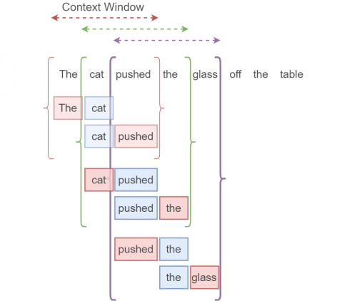
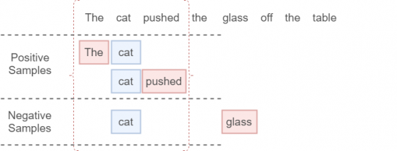
Word2vec turns a pile of unlabelled text into a supervised learning problem. It slides a window over the text and creates training pairs of a target word and a context word that appears within the window:
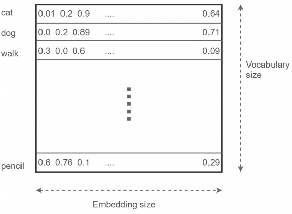
The model itself is tiny. It has an embedding layer, a table with one row per vocabulary word, initialised randomly:
Training then repeats a simple loop:
- Look up the vector of the target word in the embedding layer.
- Use it to predict the context word. In the original formulation, a softmax output layer gives a probability for every word in the vocabulary.
- Compare the prediction with the real context word using a loss function.
- Update the vectors with backpropagation and stochastic gradient descent.
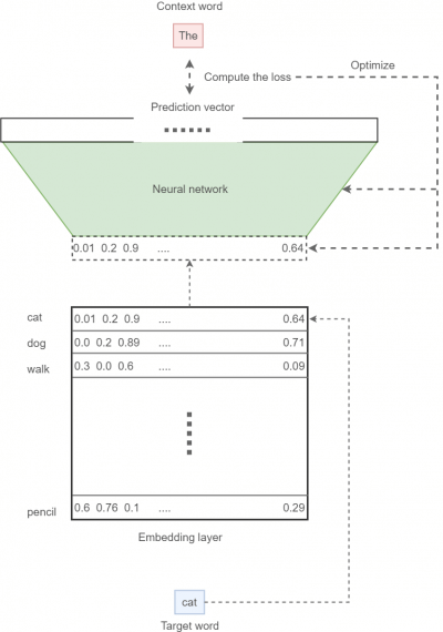
After training, the prediction layer is thrown away. What we keep is the embedding layer: the learned vectors are the product. In the language of neural networks, word2vec is a network with a single linear hidden layer whose weights are the word vectors.
CBOW vs skip-gram
Word2vec has two architectures that frame the prediction task in opposite directions:
- Continuous bag of words (CBOW) predicts the target word from the average of its context word vectors: given “the cat ___ the glass”, predict “pushed”. Averaging the context smooths the signal, so CBOW trains several times faster and works well for frequent words.
- Skip-gram does the opposite: given “pushed”, predict each word around it. Every word generates several training pairs, so training is slower, but rare words get more updates. Skip-gram usually gives better vectors for rare words and semantic relations.
| CBOW | Skip-gram | |
|---|---|---|
| Predicts | Target word from its context | Context words from the target |
| Training speed | Faster | Slower (about 3× in our test) |
| Rare words | Weaker | Better |
| Best for | Large corpora, frequent words, syntax | Smaller corpora, rare words, semantic relations |
Negative sampling and subsampling
A full softmax over the vocabulary is expensive: with 100,000 words, every training pair requires computing a score for all 100,000 of them. The second word2vec paper introduced two tricks that made training on billions of words practical.
Negative sampling turns the task into binary classification. For each real (target, context) pair, the model also draws k random “negative” words, typically 5 to 20, and learns to tell real pairs from random ones. The loss for one pair is
−log σ(vcontext · vtarget) − Σi=1..k log σ(−vnegative i · vtarget),
where σ is the sigmoid function. The first term pulls the vectors of real neighbours together; the second pushes random words away. Instead of 100,000 scores, each step needs only k + 1. Negative words are drawn in proportion to their frequency raised to the power 0.75, which gives rare words a slightly better chance than their raw frequency.
Subsampling of frequent words randomly drops very common words such as “the”, “of” and “and”, which appear in almost every window and carry little information. In our run it removed 44% of the tokens, speeding up training and improving the vectors of rarer words.
An alternative to negative sampling is hierarchical softmax, which arranges the vocabulary in a binary tree so that each prediction needs only about log2(vocabulary size) steps. Negative sampling is the more common choice today.
Word2vec from scratch in PyTorch
To see that there is no magic inside, we implemented skip-gram with negative sampling in about 50 lines of PyTorch. The corpus is text8, the first 100 MB of English Wikipedia (about 17 million words, CC BY-SA licence), a standard benchmark for word vectors. The script keeps the 71,290 words that occur at least 5 times, subsamples frequent words, builds all (target, context) pairs within a window of 5 words and trains two embedding tables: one for words as targets and one for words as context. The training step is exactly the loss formula above.
The code needs PyTorch and NumPy. Download text8.gz from the text8 release of the gensim-data repository on GitHub and unpack it into a data folder. One pass over the data took about 20 minutes on two CPU cores and needs about 4 GB of memory.
import collections

import numpy as np
import torch
from torch import nn

# 1. Corpus: text8, the first 100 MB of English Wikipedia (about 17 million words)
words = open("data/text8").read().split()
counts = collections.Counter(words)
vocab = [w for w, c in counts.most_common() if c >= 5]            # words seen at least 5 times
index = {w: i for i, w in enumerate(vocab)}
freq = np.array([counts[w] for w in vocab], dtype=np.float64)
ids = np.array([index[w] for w in words if w in index])
rng = np.random.default_rng(0)

# 2. Subsampling: randomly drop very frequent words such as "the" and "of"
p = freq[ids] / freq.sum()
ids = ids[rng.random(len(ids)) < np.sqrt(1e-4 / p) + 1e-4 / p]
print(f"vocabulary {len(vocab):,} words, {len(ids):,} tokens after subsampling")

# 3. Training pairs (target word, context word) from a window of 5 words on each side
pairs = np.concatenate([np.stack([ids[:-d], ids[d:]], 1) for d in range(1, 6)] +
                       [np.stack([ids[d:], ids[:-d]], 1) for d in range(1, 6)])
pairs = torch.from_numpy(pairs[rng.permutation(len(pairs))])
noise = torch.tensor(freq ** 0.75 / (freq ** 0.75).sum())       # negative sampling distribution
print(f"{len(pairs):,} training pairs")

# 4. Skip-gram with negative sampling: two embedding tables, nothing else
dim, negatives = 100, 5
target_emb = nn.Embedding(len(vocab), dim, sparse=True)
context_emb = nn.Embedding(len(vocab), dim, sparse=True)
nn.init.uniform_(target_emb.weight, -0.5 / dim, 0.5 / dim)
nn.init.zeros_(context_emb.weight)
opt = torch.optim.SparseAdam(list(target_emb.parameters()) + list(context_emb.parameters()), lr=0.003)

for step, batch in enumerate(pairs.split(4096)):
    t, c = target_emb(batch[:, 0]), context_emb(batch[:, 1])
    n = context_emb(torch.multinomial(noise, len(batch) * negatives, replacement=True).view(len(batch), negatives))
    pos = nn.functional.logsigmoid((t * c).sum(1))                       # real pairs: push together
    neg = nn.functional.logsigmoid(-(n @ t.unsqueeze(2)).squeeze(2)).sum(1)  # random words: push apart
    loss = -(pos + neg).mean()
    opt.zero_grad()
    loss.backward()
    opt.step()
    if step % 5000 == 0:
        print(f"step {step:6d}  loss {loss.item():.3f}")

# 5. Nearest neighbours by cosine similarity
vectors = nn.functional.normalize(target_emb.weight.detach(), dim=1)
for word in ["computer", "france", "einstein", "guitar", "happy"]:
    sims = vectors @ vectors[index[word]]
    print(f"{word:9s}", ", ".join(vocab[i] for i in sims.topk(7).indices[1:].tolist()))
vocabulary 71,290 words, 9,386,707 tokens after subsampling
93,867,040 training pairs
step 0 loss 4.159
step 5000 loss 2.360
step 10000 loss 2.326
step 15000 loss 2.281
step 20000 loss 2.251
computer computers, hardware, computing, bresenham, interfacing, microcomputer
france belgium, french, gaulle, clerc, poissy, spain
einstein relativity, dinger, podolsky, planck, electrodynamics, physics
guitar guitars, drums, bass, vocals, banjo, acoustic
happy pretty, sneer, tease, restful, laugh, crapAfter a single pass over the data, the loss fell from 4.16 to 2.25 and the vectors already make sense: the nearest neighbours of “computer” are “computers”, “hardware” and “computing”, those of “guitar” are other instruments, and those of “einstein” are “relativity”, Planck and physics. Nothing in the code knows what these words mean; the structure comes only from which words appear near which. The neighbours of “happy” are much noisier, a first sign that 17 million words of encyclopedia text contain little emotional language.
Experiment: CBOW vs skip-gram vs GloVe
In practice, nobody trains word2vec with a hand-written loop: the gensim library implements it in optimised C and trains on all CPU cores. We trained CBOW and skip-gram on text8 with typical settings (100 dimensions, a window of 5 words, 5 negative samples, 5 epochs) and evaluated both on Google’s analogy test set, 19,544 questions such as “Athens is to Greece as Oslo is to ?” (semantic) and “walking is to walked as swimming is to ?” (syntactic). For comparison we loaded pretrained GloVe vectors from Stanford, trained on 6 billion words of Wikipedia and news (Public Domain Dedication and License).
The code needs pip install gensim. The data files are the text8 and glove-wiki-gigaword-100 releases of the gensim-data repository on GitHub; unpack text8.gz into the data folder and keep the GloVe file as data/glove100.gz.
import time

from gensim.models import Word2Vec, KeyedVectors
from gensim.models.word2vec import Text8Corpus
from gensim.test.utils import datapath

# text8: the first 100 MB of English Wikipedia, about 17 million words (CC BY-SA)
corpus = Text8Corpus("data/text8")
analogies = datapath("questions-words.txt")      # Google's 19,544 analogy questions

models = {}
for name, sg in [("CBOW", 0), ("Skip-gram", 1)]:
    start = time.time()
    model = Word2Vec(corpus, vector_size=100, window=5, min_count=5, sg=sg, negative=5,
                     sample=1e-4, epochs=5, workers=2, seed=1)
    minutes = (time.time() - start) / 60
    score, sections = model.wv.evaluate_word_analogies(analogies, restrict_vocab=30000)
    semantic = sum(len(s["correct"]) for s in sections[:5]) / sum(len(s["correct"]) + len(s["incorrect"]) for s in sections[:5])
    syntactic = sum(len(s["correct"]) for s in sections[5:-1]) / sum(len(s["correct"]) + len(s["incorrect"]) for s in sections[5:-1])
    print(f"{name:9s} vocabulary {len(model.wv):,} words, trained in {minutes:.1f} min, "
          f"analogies {score:.1%} (semantic {semantic:.1%}, syntactic {syntactic:.1%})")
    models[name] = model.wv
models["Skip-gram"].save("skipgram_text8.kv")

# Pretrained GloVe vectors (Stanford), trained on 6 billion words of Wikipedia and news, for comparison
glove = KeyedVectors.load_word2vec_format("data/glove100.gz", no_header=False)
score, sections = glove.evaluate_word_analogies(analogies, restrict_vocab=30000)
print(f"GloVe 100d (6B words) analogies {score:.1%}")

wv = models["Skip-gram"]
for word in ["computer", "france", "einstein", "guitar", "happy"]:
    print(f"{word:9s}", ", ".join(w for w, _ in wv.most_similar(word, topn=6)))
for a, b, c in [("king", "man", "woman"), ("paris", "france", "germany"), ("walking", "walk", "swim"), ("bigger", "big", "small")]:
    for name, vectors in [("text8 skip-gram", wv), ("GloVe", glove)]:
        top3 = vectors.most_similar(positive=[a, c], negative=[b], topn=3)
        print(f"{a} - {b} + {c} ({name}): " + ", ".join(f"{w} {s:.2f}" for w, s in top3))
print("doesn't match:", wv.doesnt_match(["breakfast", "lunch", "dinner", "pencil"]))
CBOW vocabulary 71,290 words, trained in 1.1 min, analogies 30.7% (semantic 21.6%, syntactic 35.3%)
Skip-gram vocabulary 71,290 words, trained in 3.3 min, analogies 37.4% (semantic 31.8%, syntactic 40.2%)
GloVe 100d (6B words) analogies 65.5%
computer computers, computing, microcomputer, hardware, pdas, networked
france belgium, spain, italy, netherlands, portugal, philippe
einstein relativity, electrodynamics, bose, heisenberg, gravitation, quantum
guitar guitars, bass, banjo, drums, acoustic, percussion
happy susie, yesterday, laugh, happily, lovely, laughs
king - man + woman (text8 skip-gram): queen 0.64, daughter 0.62, princess 0.61
king - man + woman (GloVe): queen 0.77, monarch 0.68, throne 0.68
paris - france + germany (text8 skip-gram): berlin 0.83, munich 0.81, leipzig 0.75
paris - france + germany (GloVe): berlin 0.88, frankfurt 0.80, vienna 0.77
walking - walk + swim (text8 skip-gram): crawling 0.67, cages 0.66, crawl 0.63
walking - walk + swim (GloVe): swimming 0.80, surfing 0.66, swam 0.64
bigger - big + small (text8 skip-gram): smaller 0.76, larger 0.75, large 0.68
bigger - big + small (GloVe): larger 0.89, smaller 0.87, large 0.79
doesn't match: pencil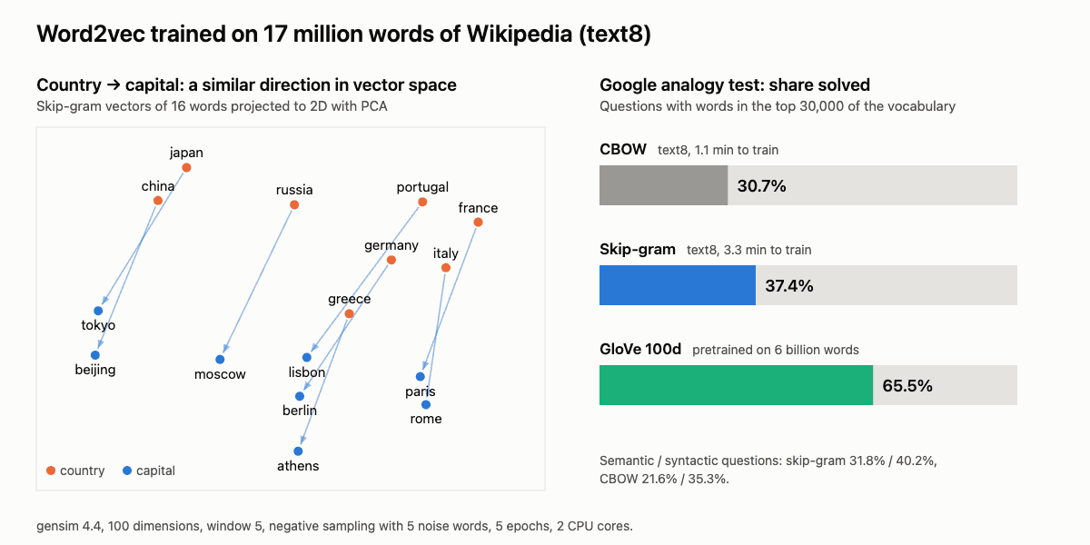
What the experiment shows:
- Skip-gram beats CBOW on meaning, CBOW wins on speed. Skip-gram solved 37.4% of the analogy questions against 30.7% for CBOW, and the gap is largest on semantic questions such as capitals and family relations (31.8% vs 21.6%). CBOW trained three times faster: 1.1 minutes against 3.3.
- Data matters more than the algorithm. GloVe vectors trained on 6 billion words solved 65.5% of the same questions. Our models saw 17 million words, about 350 times less.
- The famous analogies work, with caveats. On text8, king − man + woman gives “queen”, but “daughter” and “princess” are close behind; paris − france + germany gives “berlin” with “munich” a close second. GloVe gets these right with larger margins, and it also solves walking − walk + swim = swimming, which our small model misses.
- Neighbours reveal what the corpus is about. The neighbours of “einstein” are physics terms, because Wikipedia writes about Einstein in the context of physics. The neighbours of “happy” are noisy, because emotional words are rare in encyclopedia text. Embeddings reflect their training data, including its gaps and biases.
Results vary by about one percentage point between runs, because gensim trains with several threads. We report the output of the run shown above.
Word2vec vs GloVe, fastText and BERT
- GloVe (Global Vectors, Stanford, 2014) learns vectors from a matrix of word co-occurrence counts over the whole corpus rather than from local windows one at a time. In practice, GloVe and word2vec produce vectors of similar quality; the pretrained GloVe files are popular because they are trained on billions of words.
- fastText (Facebook AI Research, 2016) extends skip-gram by representing each word as a bag of character n-grams, so “walking” shares pieces with “walked” and “walker”. It can build vectors for words it has never seen, which helps with typos and languages with rich morphology such as Russian, Finnish or Turkish.
- Contextual embeddings (ELMo and BERT in 2018, then GPT and other transformer models) produce a different vector for each occurrence of a word depending on the sentence. “Bank” in “river bank” and in “bank account” gets different vectors. These models are far more accurate on almost every NLP task, at the cost of much more computation.
- Sentence and text embeddings from modern embedding models map whole sentences or documents to a single vector. They power semantic search, recommendation and retrieval-augmented generation (RAG), where documents are found by vector similarity; see our guide to building a private RAG pipeline.
The core idea is the same in all of them: represent meaning as a point in a vector space learned from data. Word2vec is the simplest and fastest member of the family. It trains in minutes on a laptop, needs no GPU and still works well for keyword expansion, clustering and as input features for small models.
Applications and limitations
Word2vec and similar static embeddings are used for:
- Features for NLP models: initialising the embedding layer of text classifiers, recurrent networks and LSTMs, which was standard practice from 2013 until transformers took over.
- Search and query expansion: finding synonyms and related terms to broaden a search.
- Recommendations: the same algorithm works on any sequence, not just text. Treating products in a shopping session or songs in a playlist as “words” gives item embeddings (often called item2vec or prod2vec) for recommendations.
- Clustering and visualisation of vocabularies, topics and documents.
- Studying language and society: researchers use embeddings trained on texts from different decades to measure how word meanings and associations change over time.
The main limitations:
- One vector per word. Words with several meanings get a blend of them.
- Out-of-vocabulary words. Word2vec knows nothing about words that were not in the training data (fastText partly solves this).
- Word order is ignored within the window, and phrases need special handling.
- Bias. Embeddings absorb stereotypes from their training text. A 2016 study by Tolga Bolukbasi and colleagues showed that Google News vectors completed “man is to computer programmer as woman is to ___” with “homemaker”. Any system built on embeddings should be checked for such associations.
- Analogies are imperfect. Famous examples work, but many do not, and the analogy test excludes the input words from the answers, which flatters the results.
FAQ
What is word2vec in simple terms?
Word2vec is a technique that turns each word into a list of numbers by learning from which words appear near each other in large amounts of text. Words used in similar ways get similar numbers, so a computer can measure how related two words are.
What is the difference between CBOW and skip-gram?
CBOW predicts a word from the words around it; skip-gram predicts the surrounding words from a single word. CBOW is faster, skip-gram is slower but usually better for rare words and semantic relations, as our experiment shows.
Is word2vec a neural network?
Yes, a very shallow one: an embedding layer and an output layer, with no non-linear hidden layers. Its weights are trained with backpropagation and gradient descent like any other network, and the learned weights of the first layer are the word vectors.
Is word2vec still used in 2026?
Yes, but less often as the core of NLP systems. Transformer models with contextual embeddings have replaced it for most language understanding tasks. Word2vec is still used where speed, small size and simplicity matter: keyword and product similarity, recommendations, feature engineering and teaching.
What is the difference between word2vec and BERT?
Word2vec gives every word one fixed vector, regardless of context. BERT is a deep transformer model that produces a different vector for each occurrence of a word, depending on the whole sentence. BERT is much more accurate but needs far more computation to train and run.
How many dimensions should word vectors have?
Typical values are 100 to 300. Larger vectors capture more nuance but need more data to train; for small corpora, 50 to 100 dimensions are often enough.