A recurrent neural network (RNN) is a neural network for sequential data: text, speech, time series, video. Instead of looking at each input separately, it reads a sequence one element at a time and keeps a hidden state, a memory of what it has seen so far, which it updates at every step with the same weights. This lets it use earlier words to understand later ones, predict the next value of a series or generate text character by character. RNNs and their gated versions, LSTM and GRU, were the standard models for language and speech in the 2010s, until Transformers replaced them for most of these tasks.
This guide explains how an RNN works, with the equations and a forward pass written from scratch, the main types of RNNs, how they are trained with backpropagation through time, why gradients vanish or explode, a character-level text generator in PyTorch, and how RNNs compare with CNNs and Transformers.
Key takeaways
- RNN full form: recurrent neural network. “Recurrent” means the same computation is repeated for every element of a sequence, and its result feeds into the next step.
- Core equation:
ht = tanh(Wxh xt + Whh ht−1 + b). The new hidden state depends on the current input and the previous state. - Types: one to many, many to one, many to many (encoder-decoder or synced), plus bidirectional and deep RNNs.
- Training: backpropagation through time; plain RNNs suffer from vanishing and exploding gradients, so they struggle with long-term dependencies.
- Today: LSTMs and GRUs fixed the memory problem, and Transformers took over language tasks, but recurrence is back in state space models and xLSTM.
What Is a Recurrent Neural Network?
A traditional feedforward network assumes that all inputs are independent of each other. For many tasks that is a bad assumption. To predict the next word in a sentence, you need the words before it; to recognize speech, you need the sounds that came earlier; to forecast tomorrow’s demand, you need the history of the series.
RNNs are called recurrent because they perform the same task for every element of a sequence, with the output depending on the previous computations. Another way to think about it: an RNN has a memory that captures information about what has been computed so far. The idea goes back to the 1980s; the simple form used today is often called the Elman network, after Jeffrey Elman’s 1990 paper “Finding Structure in Time”.
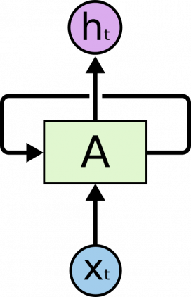
A recurrent block A takes an input xt, outputs ht and passes its state to the next step through a loop:
How an RNN Works
The loop becomes clearer if we unroll the network over time, writing out a copy for every step. For a sentence of five words, the unrolled network has five steps, one per word:
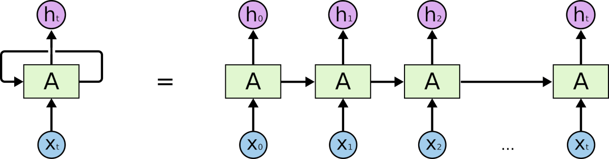
At each time step t, an RNN does two things:
ht = tanh(Wxh xt + Whh ht−1 + bh)
yt = Why ht + by
xtis the input at stept, for example a vector representing the second word of a sentence.htis the hidden state, the memory of the network. It is computed from the current input and the previous state. Thetanhactivation function keeps it between −1 and 1; ReLU is sometimes used instead. The initial stateh0is usually a vector of zeros.ytis the output at stept. To predict the next word, it is passed through softmax to get a probability for every word in the vocabulary.
Three things are worth noting:
- Parameter sharing. Unlike a deep feedforward network, which has different weights in every layer, an RNN uses the same
Wxh,WhhandWhyat every step. It performs the same task with different inputs, which greatly reduces the number of parameters and lets it process sequences of any length. - The hidden state is a summary.
htcaptures information about everything that happened before stept, but it is a fixed-size vector, so in practice it cannot hold information from too many steps back. - Outputs and inputs are optional. The diagram has an output at every step, but many tasks need only the last one. To classify the sentiment of a review, we care about the final prediction, not about the sentiment after each word.
RNN Forward Pass from Scratch
The forward pass is just a loop over the sequence. The code below implements it in NumPy and checks that it gives exactly the same hidden states as PyTorch’s nn.RNN:
import numpy as np
import torch
import torch.nn as nn

torch.manual_seed(0)
rnn = nn.RNN(input_size=3, hidden_size=5, batch_first=True)    # tanh RNN, one layer
W_xh, W_hh = rnn.weight_ih_l0.detach().numpy(), rnn.weight_hh_l0.detach().numpy()
b = (rnn.bias_ih_l0 + rnn.bias_hh_l0).detach().numpy()

def rnn_forward(xs):
    h = np.zeros(5)                                  # the initial hidden state is zero
    states = []
    for x in xs:                                     # the same weights are used at every step
        h = np.tanh(W_xh @ x + W_hh @ h + b)
        states.append(h)
    return np.stack(states)

xs = torch.randn(1, 4, 3)                            # one sequence of 4 steps, 3 features each
ours = rnn_forward(xs[0].numpy())
theirs, h_last = rnn(xs)
print("same hidden states:", np.allclose(ours, theirs[0].detach().numpy(), atol=1e-6))
print("hidden states shape:", ours.shape)
print("parameters:", sum(p.numel() for p in rnn.parameters()))
same hidden states: True
hidden states shape: (4, 5)
parameters: 50The layer has 5 · 3 input weights, 5 · 5 recurrent weights and two bias vectors of 5, which PyTorch keeps separately: 50 parameters in total, no matter how long the sequence is.
Types of RNNs
RNNs are flexible about the shape of their inputs and outputs. Andrej Karpathy’s well-known classification has five cases:
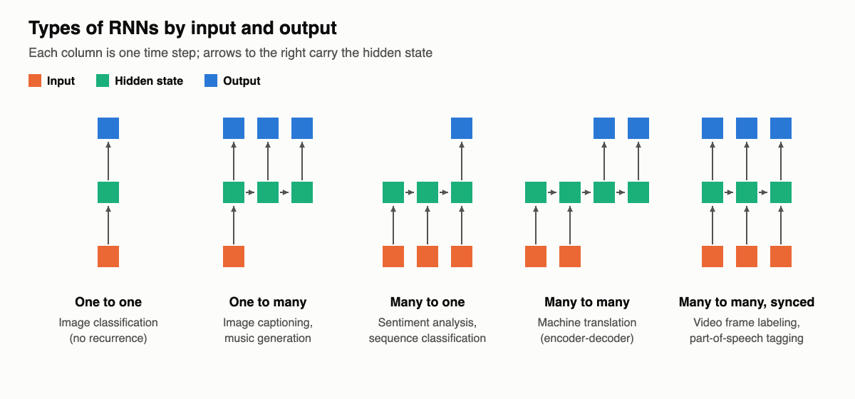
- One to one: a single input and a single output, an ordinary network with no recurrence, for example image classification.
- One to many: one input produces a sequence. Image captioning takes an image and generates a sentence word by word; music generation starts from a seed.
- Many to one: a sequence produces one output, as in sentiment analysis of a review, spam detection or classifying a time series.
- Many to many, encoder-decoder: the network reads the whole input sequence and then generates an output sequence of a different length. Machine translation works this way, because the first word of the translation may depend on the whole source sentence. These models are called sequence to sequence (seq2seq) models.
- Many to many, synced: one output for every input, for example labeling every frame of a video or tagging every word with its part of speech.
For language modeling and text generation, the RNN reads a sequence of words or characters and at every step predicts the next one, so the target sequence is the input shifted by one step. During generation, each predicted token is fed back in as the next input.
Training: Backpropagation Through Time
An RNN is trained like any other network, with backpropagation and gradient descent, with one twist. Because the same parameters are used at every step, the gradient at each output depends not only on the current step but also on all earlier ones. To compute the gradient at step t = 4, we have to propagate the error back through steps 3, 2 and 1 and sum the contributions. This is called backpropagation through time (BPTT): it is ordinary backpropagation applied to the unrolled network.
For long sequences, unrolling over thousands of steps is slow and needs a lot of memory, so in practice truncated BPTT is used: the sequence is cut into chunks of, say, 100 steps, the hidden state is carried from one chunk to the next, but gradients flow back only within a chunk. The text generator below trains on random chunks of 100 characters.
Vanishing and Exploding Gradients
Going back one step multiplies the gradient by the recurrent weight matrix Whh and by the derivative of tanh, which is at most 1. Going back k steps multiplies it by this product k times. If the factors are smaller than one, the gradient shrinks exponentially and vanishes; if they are larger, it grows exponentially and explodes. This was analyzed by Sepp Hochreiter in 1991 and by Yoshua Bengio and colleagues in 1994, and it is the central difficulty of training RNNs.
We can measure it directly. The code below builds a tanh RNN with 64 hidden units whose recurrent weights are a random orthogonal matrix times a scale, feeds it random inputs and computes how strongly the hidden state at step t still depends on the initial state:
import torch

torch.manual_seed(0)
hidden, steps = 64, 60
Q, _ = torch.linalg.qr(torch.randn(hidden, hidden))       # a random orthogonal matrix
xs = torch.randn(steps, hidden) * 0.5                       # random inputs, already multiplied by W_xh

def gradient_norms(scale):
    W_hh = scale * Q                                        # recurrent weights; scale = spectral radius
    h0 = torch.zeros(hidden, requires_grad=True)
    h, norms = h0, []
    for t in range(steps):
        h = torch.tanh(W_hh @ h + xs[t])
        # how strongly does the state at step t still depend on the initial state?
        g, = torch.autograd.grad(h.sum(), h0, retain_graph=True)
        norms.append(g.norm().item())
    return norms

for scale in (0.8, 1.0, 1.5, 2.0):
    n = gradient_norms(scale)
    print(f"scale {scale}: gradient norm after 1, 10, 30, 60 steps: "
          f"{n[0]:.1e}  {n[9]:.1e}  {n[29]:.1e}  {n[59]:.1e}")
scale 0.8: gradient norm after 1, 10, 30, 60 steps: 5.4e+00 1.0e-01 7.0e-06 6.5e-12
scale 1.0: gradient norm after 1, 10, 30, 60 steps: 6.8e+00 7.0e-01 1.9e-03 4.0e-07
scale 1.5: gradient norm after 1, 10, 30, 60 steps: 1.0e+01 1.2e+01 5.6e+00 6.1e+00
scale 2.0: gradient norm after 1, 10, 30, 60 steps: 1.4e+01 7.6e+01 9.2e+02 5.7e+03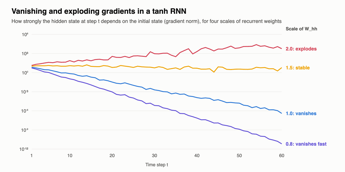
With a scale of 0.8, after 60 steps the gradient is 1012 times smaller than at the start: whatever happened 60 steps ago has no influence on learning. Even with a scale of 1.0 it vanishes, because tanh squashes it at every step. With a scale of 2.0 it grows by more than two orders of magnitude, so a single update can throw the weights far away. There is only a narrow range in between where the gradient stays stable, and the network does not stay there on its own as its weights change during training.
Common remedies:
- Gradient clipping against exploding gradients: if the gradient norm exceeds a threshold, scale it down. It is a one-line fix,
clip_grad_norm_in PyTorch, used in the example below. - Gated architectures against vanishing gradients: LSTM and GRU cells add a memory path updated by addition, so gradients can pass many steps without shrinking.
- Careful initialization, for example orthogonal or identity recurrent weights, ReLU activations with identity initialization (IRNN), and normalization layers.
- Truncated BPTT and skip connections to shorten the paths gradients have to travel.
Example: Character-Level Text Generation in PyTorch
A classic way to see what an RNN learns is a character-level language model, popularized by Andrej Karpathy’s “The Unreasonable Effectiveness of Recurrent Neural Networks”. The network reads text one character at a time and learns to predict the next character. Trained on Shakespeare, it writes Shakespeare-like text; trained on source code, it writes code. Here we train a plain RNN on 237,000 characters of Python source code from nine modules of the standard library, which every Python installation has, and then let it write code:
import os
import torch
import torch.nn as nn

# Training text: the source code of nine modules from Python's standard library
lib = os.path.dirname(os.__file__)
files = ["textwrap", "random", "statistics", "fractions", "string", "heapq", "bisect", "calendar", "shlex"]
text = "".join(open(os.path.join(lib, f + ".py"), encoding="utf-8").read() for f in files)
chars = sorted(set(text))
idx = {ch: i for i, ch in enumerate(chars)}
data = torch.tensor([idx[ch] for ch in text])
print(f"{len(text):,} characters, vocabulary of {len(chars)}")

class CharRNN(nn.Module):
    def __init__(self, vocab, hidden=256):
        super().__init__()
        self.embed = nn.Embedding(vocab, 64)
        self.rnn = nn.RNN(64, hidden, batch_first=True)    # a plain tanh RNN
        self.out = nn.Linear(hidden, vocab)

    def forward(self, x, h=None):
        y, h = self.rnn(self.embed(x), h)
        return self.out(y), h                              # next-character logits at every step

torch.manual_seed(0)
model = CharRNN(len(chars))
opt = torch.optim.Adam(model.parameters(), lr=2e-3)
seq_len = 100
for step in range(1, 3001):
    starts = torch.randint(0, len(data) - seq_len - 1, (64,))
    x = torch.stack([data[s:s + seq_len] for s in starts])           # input characters
    y = torch.stack([data[s + 1:s + seq_len + 1] for s in starts])   # targets: the next characters
    logits, _ = model(x)
    loss = nn.functional.cross_entropy(logits.reshape(-1, len(chars)), y.reshape(-1))
    opt.zero_grad()
    loss.backward()
    nn.utils.clip_grad_norm_(model.parameters(), 1.0)                  # guard against exploding gradients
    opt.step()
    if step in (1, 100, 1000, 3000):
        print(f"step {step:4d}: loss {loss.item():.2f}")

def generate(prompt, length=250, temperature=0.8):
    x = torch.tensor([[idx[ch] for ch in prompt]])
    out, h = prompt, None
    with torch.no_grad():
        for _ in range(length):
            logits, h = model(x, h)                    # the hidden state carries the context forward
            probs = torch.softmax(logits[0, -1] / temperature, dim=0)
            nxt = torch.multinomial(probs, 1).item()
            out += chars[nxt]
            x = torch.tensor([[nxt]])
    return out

torch.manual_seed(2)
print(generate("    def "))
Output (about two minutes on a CPU; the exact text depends on your Python version):
237,370 characters, vocabulary of 161
step    1: loss 5.11
step  100: loss 2.22
step 1000: loss 1.06
step 3000: loss 0.93
    def __rect_random()
                    while as the seell' > 1 is presentation_type in "we', 'red', 'by token        else:
            return result

    def __rst_ints(self, only for output follitial_indent="%s, self.firstweekday", "heapify() methods.y
The loss falls from 5.1, random guessing among 161 characters, to 0.93. After a few minutes of training, the network has learned the shape of Python on its own: indentation, def and self, method names with double underscores, quotes and brackets that come in pairs, return statements, even words from docstrings. It has no idea what the code means, and it does not know words or syntax rules: everything comes from predicting one character at a time with a hidden state of 256 numbers.
The temperature controls how adventurous the sampling is: lower values make the model pick the most likely characters and repeat itself, higher values make the text more varied and more broken. A larger model, an LSTM instead of a plain RNN and more training produce much more convincing results.
RNN Architectures: Bidirectional, Deep, LSTM and GRU
Over the years, researchers developed more advanced types of RNNs to fix the weaknesses of the simple model:
- Bidirectional RNNs, proposed by Mike Schuster and Kuldip Paliwal in 1997, are based on the idea that the output at time
tmay depend on future elements as well as past ones. To fill in a missing word, you want both the left and the right context. A bidirectional RNN is simply two RNNs, one reading the sequence forward and one backward, whose hidden states are combined at every step. It can only be used when the whole sequence is available, not for real-time prediction. - Deep (stacked) RNNs put several recurrent layers on top of each other, each taking the hidden states of the layer below as its input. They have more capacity but need more data to train.
- LSTM networks keep the same chain structure but compute the hidden state differently. Each cell has a separate cell state and three gates that decide what to keep, what to write and what to output, which makes it far better at long-term dependencies. Our LSTM guide explains it step by step and compares it with a plain RNN in an experiment.
- GRU (gated recurrent unit), introduced in 2014, is a simpler gated cell with two gates and no separate cell state; it performs about as well as an LSTM on most tasks.
- Encoder-decoder RNNs with attention. Sequence-to-sequence models compress the input into one vector, which is a bottleneck for long sentences. In 2014 Dzmitry Bahdanau, Kyunghyun Cho and Yoshua Bengio let the decoder look back at all encoder states with an attention mechanism, the idea that later became the basis of Transformers.
- Echo state networks and other reservoir computing models use a fixed random recurrent network and train only the output layer, which avoids BPTT altogether.
RNN vs CNN vs Transformer
| RNN | CNN | Transformer | |
|---|---|---|---|
| Best for | Sequences, streaming data | Images, grid-like data, local patterns | Sequences of all kinds, especially language |
| How it sees context | Through a hidden state passed step by step | Through a local receptive field that grows with depth | Through attention to every position at once |
| Parallel training | No, steps are sequential | Yes | Yes |
| Long-range dependencies | Weak (plain RNN), better with LSTM and GRU | Limited by receptive field | Strong, limited by context length |
| Cost per step at inference | Constant | Constant for fixed-size input | Grows with context length |
| Input length | Any | Usually fixed | Up to the context window |
A convolutional neural network shares weights across space, an RNN shares them across time. The two are often combined: in image captioning, a CNN encodes the image and an RNN generates the description; in video models, a CNN processes each frame and an RNN models the sequence of frames.
Transformers, introduced in 2017, replaced RNNs in machine translation, language modeling and most of speech recognition, mainly because they can be trained in parallel on huge datasets. But recurrence has advantages that Transformers lack: a fixed memory per step and natural handling of endless streams. Since 2023 new recurrent architectures, such as the state space model Mamba, RWKV and xLSTM, have combined parallel training with recurrent inference and rival Transformers of similar size on some benchmarks.
Applications of RNNs
- Language modeling and text generation. Given a sequence of words, predict the probability of each next word. RNN language models, such as Tomáš Mikolov’s RNNLM from 2010, scored how likely a sentence is, which helped speech recognition and translation choose the most fluent output, and generated new text by sampling.
- Machine translation. Encoder-decoder RNNs, introduced by Ilya Sutskever, Oriol Vinyals and Quoc Le and by Cho and colleagues in 2014, translated whole sentences end to end; Google Translate switched to an LSTM-based system in 2016.
- Speech recognition. From a sequence of acoustic features, predict a sequence of phonetic units or characters with their probabilities.
- Image captioning. Together with CNNs, RNNs generated descriptions of images, as in Andrej Karpathy and Fei-Fei Li’s “Deep Visual-Semantic Alignments for Generating Image Descriptions”.
- Time series forecasting and anomaly detection in finance, energy, sensors and logs.
- Music generation, handwriting recognition and synthesis, video analysis.
FAQ
What is the full form of RNN?
RNN stands for recurrent neural network: a neural network with a loop that passes its hidden state from one step of a sequence to the next.
What is an RNN in simple terms?
It is a network that reads data one piece at a time, like a person reading a sentence word by word, and keeps a running memory of what it has read. At each step it combines the new piece with that memory, which lets it make predictions that depend on context.
What is the difference between an RNN and an LSTM?
An LSTM is a type of RNN. A plain RNN updates its hidden state with a single tanh layer, so information and gradients fade after a few dozen steps. An LSTM adds a cell state and gates that control what to keep and forget, so it can remember information for hundreds of steps.
What is the difference between an RNN and a CNN?
A CNN processes grid-like data such as images, sharing weights across positions and detecting local patterns. An RNN processes sequences, sharing weights across time steps and carrying a hidden state forward. CNNs see a fixed-size input at once; RNNs read sequences of any length step by step.
Why do RNNs have vanishing gradients?
During backpropagation through time, the gradient is multiplied by the recurrent weights and the derivative of the activation once for every step it goes back. When these factors are smaller than one, the product shrinks exponentially, so the network cannot learn from events far in the past.
Are RNNs still used?
Yes, though less than before. Large language models are Transformers, but LSTMs and GRUs are still common for time series, small sequence tasks and on-device speech, and recurrent ideas are returning in state space models such as Mamba and in xLSTM.
Is an RNN supervised or unsupervised?
An RNN is an architecture, not a learning method. It is usually trained with supervised learning, and language models such as the text generator above are trained in a self-supervised way, using the next character of the text as the label. See our guide to supervised, unsupervised and reinforcement learning.
See also: our guides to LSTM networks, the most popular kind of RNN, and to backpropagation, the algorithm behind BPTT.