PyTorch Tutorial for Beginners: From Installation to Your First Neural Network

PyTorch is the most widely used deep learning framework in 2026: it powers most research papers, almost all open large language models and the tools around them, from Hugging Face Transformers to vLLM. It is popular because it feels like ordinary Python: you create tensors, call functions, write loops, and PyTorch computes gradients for you.

This tutorial takes you from installation to a trained neural network. You will install PyTorch with or without a GPU, learn tensors and automatic differentiation, build a small convolutional network with nn.Module, load data with Dataset and DataLoader, write a training loop, save and load the model, and speed it up with torch.compile. Every code block below was run with PyTorch 2.14 and the output is shown as printed. The data set ships with scikit-learn, so nothing needs to be downloaded.

What is PyTorch?

PyTorch is an open-source deep learning framework for Python. Facebook AI Research released it in 2016 as a Python successor to the Lua-based Torch library; version 1.0, which merged in Caffe2 for production use, followed in 2018, and since 2022 the project has been run by the PyTorch Foundation under the Linux Foundation. The current version, 2.15, was released on October 28, 2026.

PyTorch gives you three things: tensors, which are multidimensional arrays that run on CPUs and GPUs; automatic differentiation, which computes gradients of any computation; and building blocks for neural networks — layers, loss functions, optimizers and data loading utilities. Around it there is a large ecosystem: torchvision and torchaudio for images and sound, Hugging Face Transformers for language models, PyTorch Lightning for organizing training code, ExecuTorch for phones.

How to install PyTorch

PyTorch is installed with pip. The package is called torch:

pip install torch

What you get depends on the platform:

• Linux: the default wheel from PyPI already includes CUDA support for NVIDIA GPUs.
• Windows: the default wheel is CPU-only. For an NVIDIA GPU, open the selector on pytorch.org, choose your CUDA version and run the command it shows, which adds --index-url https://download.pytorch.org/whl/cu1XX.
• macOS: the default wheel supports Apple Silicon GPUs through the MPS backend.
• AMD GPUs: choose a ROCm build in the selector (Linux).

Things to check before installing:

• Python version. PyTorch 2.15 supports Python 3.11 and newer; 2.14 was the last release for Python 3.10.
• Old NVIDIA GPUs. Starting with 2.15, prebuilt CUDA wheels no longer support Maxwell, Pascal and Volta GPUs (for example GTX 10-series cards and the Tesla V100). The oldest supported generation is Turing (RTX 20-series, T4).
• Conda. PyTorch no longer publishes official conda packages. You can still use a conda environment, but install PyTorch inside it with pip.
• A virtual environment (python -m venv .venv) keeps PyTorch and its large CUDA libraries separate from other projects.

To check the installation and see whether a GPU is available:

python -c "import torch; print(torch.__version__, torch.cuda.is_available())"

If torch.cuda.is_available() prints False on a machine with an NVIDIA GPU, the usual reasons are a CPU-only wheel or an outdated NVIDIA driver. No GPU at all is fine for learning: everything in this tutorial runs on a CPU in seconds. When you need more power, see our guides to the best GPU for AI.

Tensors

A tensor is PyTorch’s basic data structure: a multidimensional array of numbers, like a NumPy array, that can also live on a GPU and track gradients. Creating tensors, doing arithmetic, indexing and moving data between NumPy and PyTorch:

import numpy as np
import torch

# Creating tensors
a = torch.zeros(2, 3)                       # 2 rows, 3 columns of zeros
b = torch.rand(2, 3)                        # uniform random numbers in [0, 1)
c = torch.tensor([[1.0, 2.0, 3.0],
                  [4.0, 5.0, 6.0]])         # from a Python list
print(a.shape, a.dtype, c.device)

# Arithmetic works element by element, @ is matrix multiplication
print(c + 1)
print(c * c)
print(c @ c.T)                              # (2x3) @ (3x2) -> 2x2

# Indexing and reshaping work like in NumPy
print(c[:, 1])                              # second column
print(c.reshape(3, 2))
print(c.sum(), c.mean(dim=0))               # reductions

# NumPy interop: from_numpy shares memory with the array
arr = np.arange(4.0)
t = torch.from_numpy(arr)
t[0] = 100
print(arr, t.numpy())

# Move a tensor to the GPU when one is available
device = "cuda" if torch.cuda.is_available() else "mps" if torch.backends.mps.is_available() else "cpu"
print("device:", device, c.to(device).device)

torch.Size([2, 3]) torch.float32 cpu
tensor([[2., 3., 4.],
        [5., 6., 7.]])
tensor([[ 1.,  4.,  9.],
        [16., 25., 36.]])
tensor([[14., 32.],
        [32., 77.]])
tensor([2., 5.])
tensor([[1., 2.],
        [3., 4.],
        [5., 6.]])
tensor(21.) tensor([2.5000, 3.5000, 4.5000])
[100.   1.   2.   3.] [100.   1.   2.   3.]
device: cpu cpu

A few things to remember. Every tensor has a shape, a dtype (usually float32 for model inputs and weights, int64 for class labels) and a device. Operations between tensors require them to be on the same device, which is the most common beginner error on GPUs. torch.from_numpy shares memory with the NumPy array, so changing one changes the other, as the output shows.

Computational graphs and autograd

Deep learning frameworks represent a computation as a graph: nodes are operations, edges carry tensors between them. Here is the graph for the expression a = (b + c) × (c + 2), split into intermediate steps d = b + c and e = c + 2:

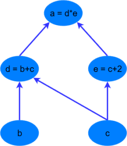
PyTorch builds this graph on the fly while your code runs, which is called a dynamic graph, and walks it backwards to compute gradients when you call .backward(). This is backpropagation, done automatically. The same expression in code:

import torch

# a = (b + c) * (c + 2), the computational graph from the picture above
b = torch.tensor(2.0, requires_grad=True)
c = torch.tensor(1.0, requires_grad=True)
d = b + c                 # intermediate node
e = c + 2                 # intermediate node
a = d * e
print("a =", a.item())

a.backward()              # walk the graph backwards and fill .grad of every leaf
print("da/db =", b.grad.item())   # = e = c + 2
print("da/dc =", c.grad.item())   # = e + d = (c + 2) + (b + c)
print("graph:", type(a.grad_fn).__name__, "<-", [type(f).__name__ for f, _ in a.grad_fn.next_functions])

a = 9.0
da/db = 3.0
da/dc = 6.0
graph: MulBackward0 <- ['AddBackward0', 'AddBackward0']

The results match the derivatives by hand: ∂a/∂b = c + 2 = 3 and ∂a/∂c = (c + 2) + (b + c) = 6. Tensors created with requires_grad=True are leaves of the graph, and after backward() their gradients are stored in .grad. In a neural network the leaves are the weights, and the gradients tell gradient descent how to change them. Older tutorials, including the 2018 version of this one, wrapped tensors in Variable objects for this; that API was merged into tensors in PyTorch 0.4 and is no longer needed.

Loading data: Dataset and DataLoader

PyTorch separates storing data from feeding it to the model. A Dataset knows how many examples there are and how to return one by index; a DataLoader groups examples into batches, shuffles them and can load them in parallel worker processes. For our example we use the digits data set from scikit-learn: 1,797 grayscale images of handwritten digits, 8×8 pixels each. In the full script below, the DigitsDataset class converts the images to a tensor of shape (N, 1, 8, 8) — number of images, channels, height, width — which is the layout convolutional layers expect. For your own data you write the same three methods, __init__, __len__ and __getitem__, typically reading image files or rows of a table in __getitem__.

Building a neural network with nn.Module

A model in PyTorch is a class that inherits from nn.Module: layers are created in __init__, and forward describes how input flows through them. The 2018 version of this tutorial built a fully connected network for 28×28 MNIST images — 784 inputs, two hidden layers of 200 neurons and 10 outputs, a classic multilayer perceptron:

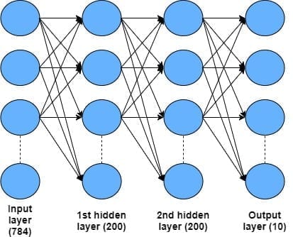
For images a convolutional neural network works better, so our DigitNet uses two convolutional layers with ReLU activations and max pooling, followed by two fully connected layers. The comments in the code track the shape of the data after every layer: 1×8×8 → 16×8×8 → 16×4×4 → 32×4×4 → 32×2×2 → 128 → 64 → 10 scores, one per digit. The whole network has 13,706 trainable parameters. You never call forward directly: calling model(x) runs it.

The training loop

Here is the complete script: data, model, training and evaluation loops, saving and loading. It runs in a few seconds on a CPU and uses a GPU automatically when one is available:

import json
import torch
from torch import nn
from torch.utils.data import Dataset, DataLoader
from sklearn.datasets import load_digits
from sklearn.model_selection import train_test_split

torch.manual_seed(0)
device = "cuda" if torch.cuda.is_available() else "mps" if torch.backends.mps.is_available() else "cpu"

# 1. Data: 1,797 grayscale images of handwritten digits, 8x8 pixels
X, y = load_digits(return_X_y=True)
X_train, X_val, y_train, y_val = train_test_split(X, y, test_size=0.2, random_state=0, stratify=y)

class DigitsDataset(Dataset):
    def __init__(self, X, y):
        self.X = torch.tensor(X / 16.0, dtype=torch.float32).reshape(-1, 1, 8, 8)  # N x channels x H x W
        self.y = torch.tensor(y, dtype=torch.long)

    def __len__(self):
        return len(self.y)

    def __getitem__(self, i):
        return self.X[i], self.y[i]

train_loader = DataLoader(DigitsDataset(X_train, y_train), batch_size=64, shuffle=True)
val_loader = DataLoader(DigitsDataset(X_val, y_val), batch_size=256)

# 2. Model: a small convolutional network
class DigitNet(nn.Module):
    def __init__(self):
        super().__init__()
        self.features = nn.Sequential(
            nn.Conv2d(1, 16, kernel_size=3, padding=1), nn.ReLU(),    # 16 x 8 x 8
            nn.MaxPool2d(2),                                          # 16 x 4 x 4
            nn.Conv2d(16, 32, kernel_size=3, padding=1), nn.ReLU(),   # 32 x 4 x 4
            nn.MaxPool2d(2),                                          # 32 x 2 x 2
        )
        self.classifier = nn.Sequential(nn.Flatten(), nn.Linear(32 * 2 * 2, 64), nn.ReLU(), nn.Linear(64, 10))

    def forward(self, x):
        return self.classifier(self.features(x))

model = DigitNet().to(device)
print("parameters:", sum(p.numel() for p in model.parameters()))
loss_fn = nn.CrossEntropyLoss()
optimizer = torch.optim.Adam(model.parameters(), lr=1e-3)

# 3. Training and evaluation loops
def train_one_epoch():
    model.train()
    total = 0.0
    for xb, yb in train_loader:
        xb, yb = xb.to(device), yb.to(device)
        loss = loss_fn(model(xb), yb)      # forward pass
        optimizer.zero_grad()              # clear old gradients
        loss.backward()                    # backpropagation
        optimizer.step()                   # update the weights
        total += loss.item() * len(yb)
    return total / len(train_loader.dataset)

@torch.no_grad()
def evaluate():
    model.eval()
    correct = 0
    for xb, yb in val_loader:
        xb, yb = xb.to(device), yb.to(device)
        correct += (model(xb).argmax(dim=1) == yb).sum().item()
    return correct / len(val_loader.dataset)

history = []
for epoch in range(1, 21):
    train_loss = train_one_epoch()
    val_acc = evaluate()
    history.append((train_loss, val_acc))
    if epoch in (1, 2, 5, 10, 15, 20):
        print(f"epoch {epoch:2d}  train loss {train_loss:.4f}  val accuracy {val_acc:.3f}")

# 4. Save the weights, load them into a new model and predict one image
torch.save(model.state_dict(), "digitnet.pt")
restored = DigitNet().to(device)
restored.load_state_dict(torch.load("digitnet.pt", map_location=device))
restored.eval()
with torch.no_grad():
    image, label = val_loader.dataset[0]
    probs = torch.softmax(restored(image.unsqueeze(0).to(device)), dim=1)[0]
print(f"true label {label.item()}, predicted {probs.argmax().item()} with probability {probs.max().item():.3f}")
json.dump(history, open("history.json", "w"))

parameters: 13706
epoch  1  train loss 2.2875  val accuracy 0.136
epoch  2  train loss 2.1887  val accuracy 0.536
epoch  5  train loss 0.7820  val accuracy 0.850
epoch 10  train loss 0.2205  val accuracy 0.914
epoch 15  train loss 0.1175  val accuracy 0.961
epoch 20  train loss 0.0743  val accuracy 0.964
true label 7, predicted 7 with probability 0.995

The heart of the script is the inner loop of train_one_epoch, the same in every PyTorch project:

1. Forward pass: model(xb) computes predictions for a batch, and the loss function compares them with the labels. CrossEntropyLoss takes raw scores (logits) and integer class labels; do not add a softmax layer before it.
2. optimizer.zero_grad() clears the gradients from the previous step; PyTorch accumulates gradients by default.
3. loss.backward() computes the gradient of the loss for all 13,706 parameters.
4. optimizer.step() updates the weights; Adam with learning rate 0.001 is a reliable default.

Two more details matter. model.train() and model.eval() switch layers such as dropout and batch normalization between training and inference behaviour. And @torch.no_grad() on the evaluation function turns off gradient tracking, which saves memory and time when you only need predictions. One pass over the training data is an epoch; with 1,437 training images and batches of 64, each epoch has 23 iterations.

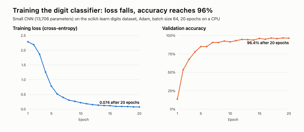
After the first epoch the network is still guessing (13.6% validation accuracy, close to the 10% of random choice among ten digits). By epoch 5 it recognizes 85% of new digits, by epoch 15 over 96%, and after 20 epochs it reaches 96.4% while the training loss drops from 2.29 to 0.074. Training longer would push the training loss lower but not the validation accuracy much higher; watching both is how you notice overfitting.

Saving, loading and predicting

The recommended way to save a model is to save its state_dict, a dictionary with all the weights: torch.save(model.state_dict(), "digitnet.pt"). To load it, create a model of the same class and call load_state_dict, as the end of the script does; map_location lets you load weights saved on a GPU into a CPU-only machine. Since PyTorch 2.6, torch.load loads only tensors and simple types by default (weights_only=True), which protects you from running code hidden in a downloaded checkpoint.

For a prediction, put the model in evaluation mode, add a batch dimension with unsqueeze(0) and convert the scores into probabilities with softmax. The restored model recognized the first validation image, a 7, with probability 0.995. For deployment outside Python, export the model with torch.export or to ONNX, or run it on phones with ExecuTorch.

Making it faster: GPU, mixed precision and torch.compile

Three changes give most of the speed in real projects:

• Use a GPU. Pick the device once, device = "cuda" (or "mps" on a Mac), and move both the model (model.to(device)) and every batch to it, as the script does. On a GPU, a large model trains tens of times faster than on a CPU.
• Mixed precision. Wrapping the forward pass in with torch.autocast(device_type="cuda", dtype=torch.bfloat16): runs most operations in 16-bit precision on tensor cores, often doubling speed and halving memory with no loss of accuracy on modern NVIDIA GPUs.
• torch.compile. One line, model = torch.compile(model), compiles the model into optimized kernels. The first call is slow because compilation happens then; after that, the compiled model runs faster.

A quick check of torch.compile on a two-layer network with 8.4 million parameters, running a batch of 256 inputs:

import time
import torch
from torch import nn

model = nn.Sequential(nn.Linear(1024, 4096), nn.GELU(), nn.Linear(4096, 1024)).eval()
x = torch.randn(256, 1024)

compiled = torch.compile(model)            # same model, compiled with TorchInductor

def bench(f, n=50):
    with torch.no_grad():
        f(x)                                # warm-up (for the compiled model: compilation happens here)
        start = time.perf_counter()
        for _ in range(n):
            f(x)
    return (time.perf_counter() - start) / n * 1000

with torch.no_grad():
    print("same output:", torch.allclose(model(x), compiled(x), atol=1e-4))
print(f"eager:    {bench(model):.2f} ms per batch")
print(f"compiled: {bench(compiled):.2f} ms per batch")

same output: True
eager:    27.34 ms per batch
compiled: 24.18 ms per batch

The compiled model gives the same output and is about 12% faster in this run. On our small two-core CPU, though, the result varied a lot between runs, from a 15% speedup to a small slowdown; on GPUs, where compilation fuses many small operations and saves memory traffic, the speedup is usually larger. Measure it on your own model, because the benefit depends heavily on the architecture.

Where to go next

• Bigger data sets and pretrained models: torchvision provides MNIST, CIFAR-10, ImageNet loaders and pretrained networks such as ResNet; for text, start with Hugging Face Transformers.
• Less boilerplate: PyTorch Lightning or Hugging Face Accelerate handle training loops, logging, checkpoints and multi-GPU training for you.
• More architectures, with PyTorch code: CNN, RNN, LSTM, variational autoencoder and GAN.
• Visualize training: torch.utils.tensorboard writes logs for TensorBoard; Weights & Biases and MLflow are popular alternatives.

FAQ

Is PyTorch hard to learn?

Not if you know Python and NumPy. The core ideas — tensors, autograd, nn.Module, a training loop — fit into this one tutorial, and the code reads like ordinary Python. What takes longer is the deep learning itself: choosing architectures, tuning learning rates, spotting overfitting.

Do I need a GPU to learn PyTorch?

No. Everything in this tutorial runs on a laptop CPU. For bigger models, free notebooks such as Google Colab and Kaggle give limited GPU time, and cloud GPUs can be rented by the hour.

How do I install PyTorch with CUDA?

On Linux, pip install torch already includes CUDA. On Windows, use the command from the selector on pytorch.org with the --index-url for your CUDA version. Then check torch.cuda.is_available(); if it prints False, update the NVIDIA driver or reinstall with the CUDA wheel.

What is the difference between torch and PyTorch?

None: PyTorch is the project’s name, torch is the name of the Python package you install and import. torchvision and torchaudio are separate companion packages.

Should I learn PyTorch or TensorFlow?

PyTorch. It is used far more widely in 2026, and since March 2026 Google maintains TensorFlow only with security and critical fixes, recommending Keras 3, JAX or PyTorch for new generative AI projects.

What is PyTorch Lightning?

A library on top of PyTorch that organizes the training loop for you: you define the model, the training step and the optimizer, and Lightning handles epochs, devices, logging, checkpoints and distributed training. It is worth learning after you have written a few training loops by hand, as in this tutorial.