Long short-term memory (LSTM) is a type of recurrent neural network designed to remember information over long sequences. An ordinary recurrent network forgets quickly: the influence of an input fades after a few dozen steps because gradients vanish during training. An LSTM adds a separate memory, the cell state, and three gates that decide what to forget, what to write and what to output at every step. This simple change made LSTMs the standard model for speech recognition, machine translation, handwriting recognition and time series forecasting through the 2010s, until Transformers took over most language tasks.
This guide explains how an LSTM works step by step, with the diagrams from Christopher Olah’s classic explanation, the equations behind each gate, an LSTM cell written from scratch and checked against PyTorch, an experiment that shows when an LSTM remembers and a plain RNN does not, a time series forecasting example, and a comparison with GRUs and Transformers.
Key takeaways
- LSTM full form: long short-term memory. It was introduced by Sepp Hochreiter and Jürgen Schmidhuber in 1997.
- Problem it solves: plain RNNs cannot learn long-term dependencies because gradients shrink exponentially as they flow back through time.
- Architecture: a cell state that runs through the whole sequence, plus forget, input and output gates, each a sigmoid layer that scales information between 0 and 1.
- Key equation:
Ct = ft · Ct−1 + it · C̃t. Memory is updated by addition, so information and gradients can pass many steps almost unchanged. - Today: Transformers dominate language modeling, but LSTMs are still used for time series, on-device speech and small sequential models, and the xLSTM architecture revived the idea in 2024.
Recurrent Neural Networks
People do not start thinking from scratch every second. As you read this sentence, you understand each word based on the words before it. A standard feedforward network cannot do that: it treats each input independently. If you wanted to classify what happens at every moment of a film, it is unclear how such a network could use earlier scenes to understand later ones.
Recurrent neural networks (RNNs) solve this with a loop. A block of the network A takes an input xt, outputs a value ht, and passes information on to the next step:
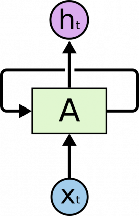
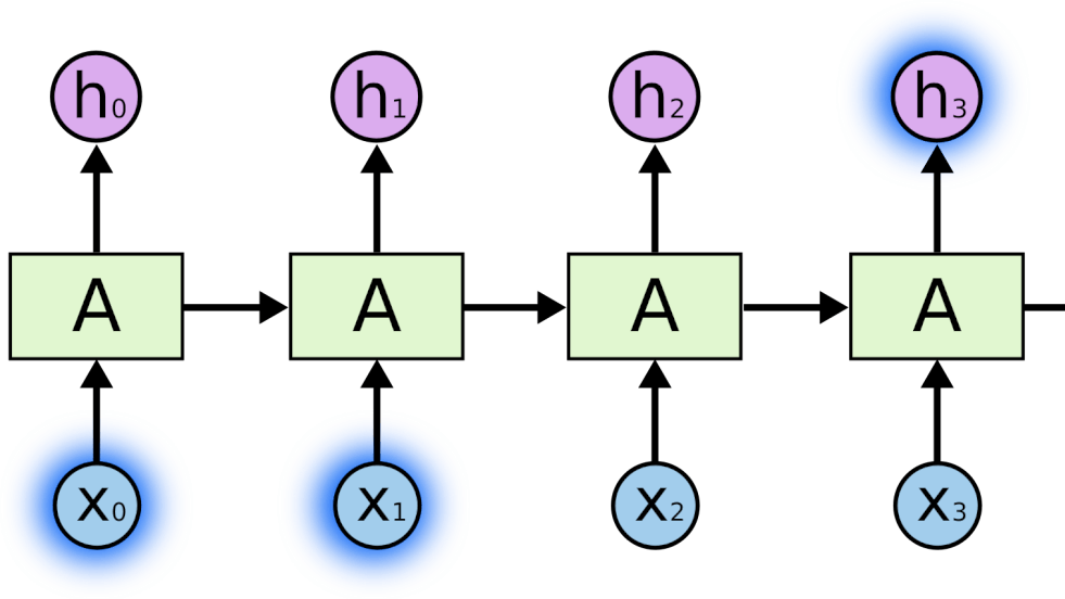
The loop looks mysterious, but an RNN is just several copies of the same network, each passing a message to its successor. Unrolled over time, it becomes a chain:
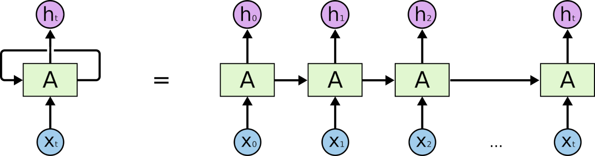
This chain structure makes RNNs a natural fit for sequences: text, speech, sensor readings, prices, video frames. At every step the network combines the new input with its hidden state, a vector that summarizes what it has seen so far, and it uses the same weights at every step. Training unrolls the chain and applies backpropagation through all the steps, which is called backpropagation through time.
The Problem of Long-Term Dependencies
The promise of RNNs is that they can connect earlier information with the present. Sometimes only recent information is needed. To predict the last word in “the clouds are in the sky“, you need no further context: the gap between the relevant words and the place where they are needed is small, and an RNN learns this easily.
Sometimes more context is needed. In “I grew up in France… I speak fluent French“, the nearby words suggest that the next word is a language, but to name the right one, the network must remember “France” from much earlier. As the gap grows, plain RNNs become unable to connect the information.
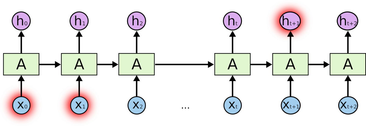
In theory an RNN can handle such long-term dependencies. In practice it cannot learn them, as Sepp Hochreiter showed in his 1991 thesis and Yoshua Bengio and colleagues in 1994. The reason is the vanishing gradient problem. The gradient that tells the network how to change its weights is multiplied by the same recurrent weights and by the derivative of tanh once for every step it travels back. When these factors are smaller than one, which they usually are, the gradient shrinks exponentially: after 50 steps almost nothing is left, so the network cannot learn that an input 50 steps ago mattered. When the factors are larger than one, gradients explode instead, which is usually handled by gradient clipping.
What Is an LSTM?
LSTM stands for long short-term memory: the network has a short-term memory, the hidden state, that lasts for a long time. LSTMs were introduced by Hochreiter and Schmidhuber in 1997 specifically to fix the long-term dependency problem. They are built so that remembering is easy: the memory is carried from step to step by addition rather than rewritten, so information can pass through unchanged. The original design always kept its memory; Felix Gers and co-authors added the forget gate in 1999–2000, letting the network also clear what it no longer needs, and this is the architecture used today.
Over the following two decades LSTMs became the workhorse of sequence modeling: speech recognition in Google’s voice search and Android, Google Translate’s neural system from 2016, handwriting recognition, text generation, music and the game-playing agents OpenAI Five and DeepMind’s AlphaStar.
LSTM Architecture
All recurrent networks are a chain of repeating modules. In a standard RNN the module is very simple, for example a single tanh layer:
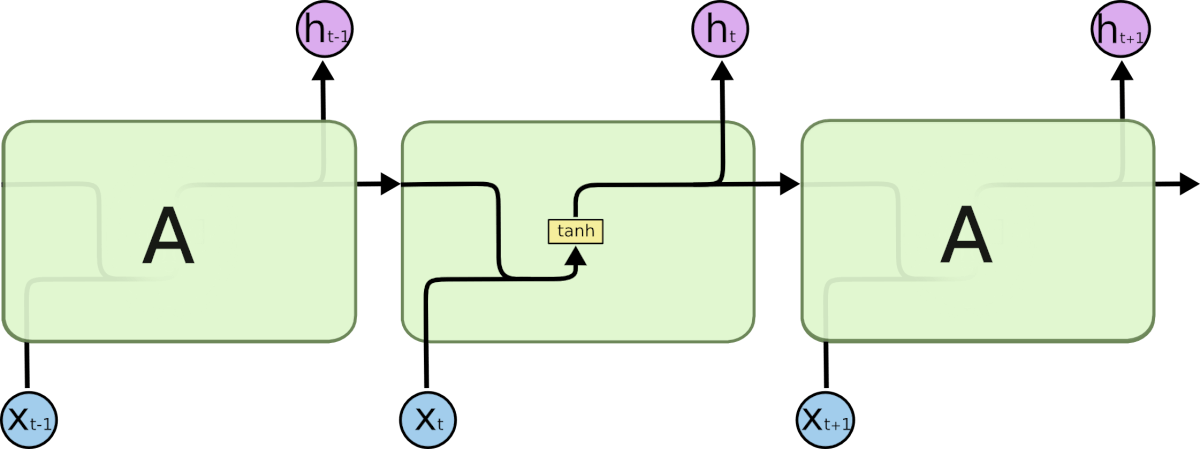
An LSTM has the same chain structure, but its repeating module has four layers that interact in a special way:
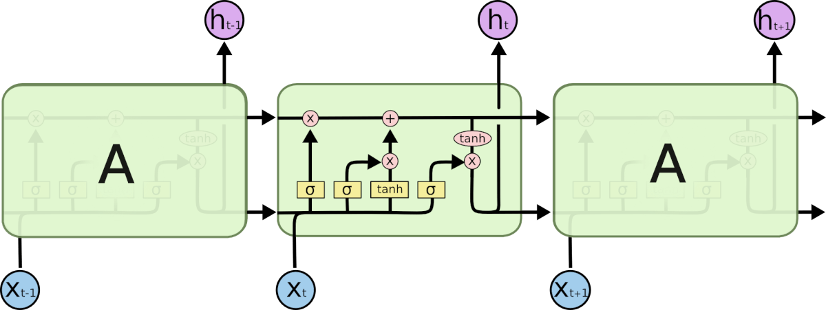
Do not worry about the details yet. In the diagrams, each line carries a vector from one node to another. Pink circles are pointwise operations, such as vector addition; yellow boxes are learned neural network layers. Lines merging means concatenation, and a line forking means its content is copied and sent to different places:

The cell state
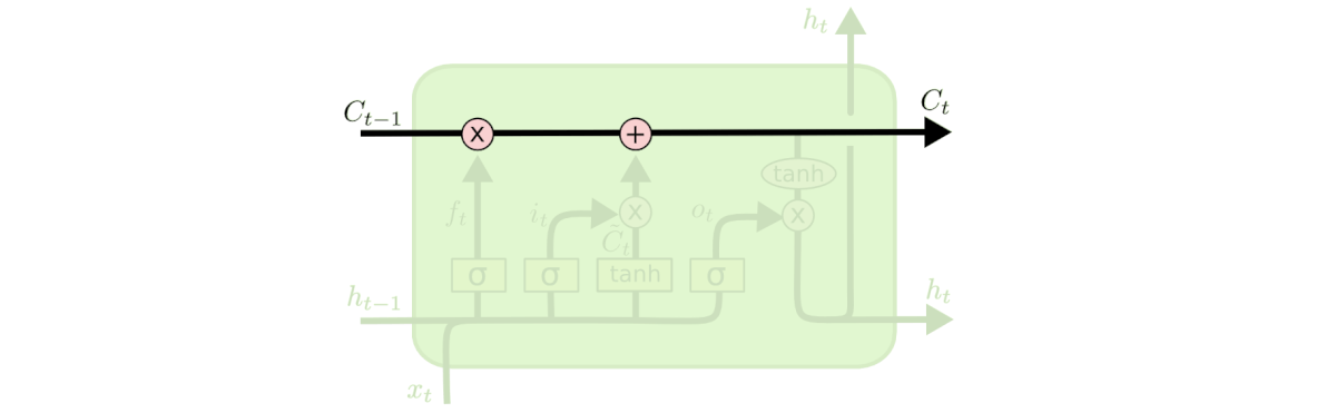
The key to LSTMs is the cell state, the horizontal line running through the top of the diagram. It works like a conveyor belt: it runs down the entire chain with only minor linear interactions, so information can flow along it unchanged.
Gates
The LSTM can remove information from the cell state or add to it, and this is regulated by structures called gates. A gate is a sigmoid layer followed by pointwise multiplication:
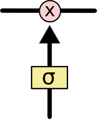
The sigmoid outputs numbers between 0 and 1 for every component of the vector, describing how much of each component to let through: 0 means “let nothing through”, 1 means “let everything through”. An LSTM has three gates that protect and control the cell state.
How an LSTM Works Step by Step
We will follow one step of an LSTM language model that reads a text and predicts the next word. Suppose its cell state stores the grammatical properties of the current subject, such as whether it is singular or plural, so that it can choose the correct verb form.
1. Forget gate: what to throw away
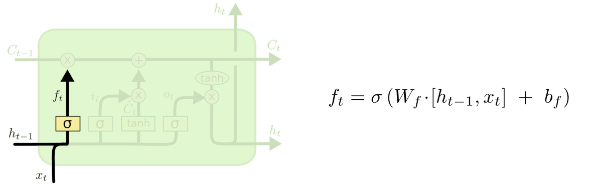
First, the LSTM decides what to remove from the cell state. The forget gate looks at the previous hidden state ht−1 and the input xt and outputs a number between 0 and 1 for each number in the cell state Ct−1: 1 means “keep this completely”, 0 means “get rid of it”. When the model sees a new subject, it should forget the properties of the old one.
2. Input gate: what new information to store
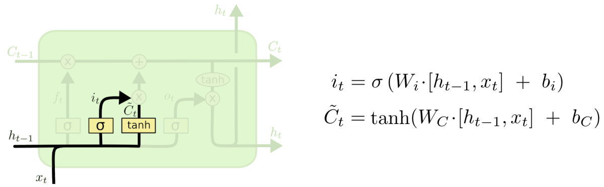
Next, the LSTM decides what new information to write. This has two parts. A sigmoid layer, the input gate it, decides which values to update. A tanh layer creates a vector of new candidate values C̃t in the range −1 to 1. In the language model, this is where the properties of the new subject are prepared.
3. Updating the cell state
Now the old cell state Ct−1 is updated to the new one, Ct. The LSTM multiplies the old state by ft, forgetting what it decided to forget, and adds it · C̃t, the new candidates scaled by how much each should be updated. The information about the old subject is dropped and the new subject is written in.
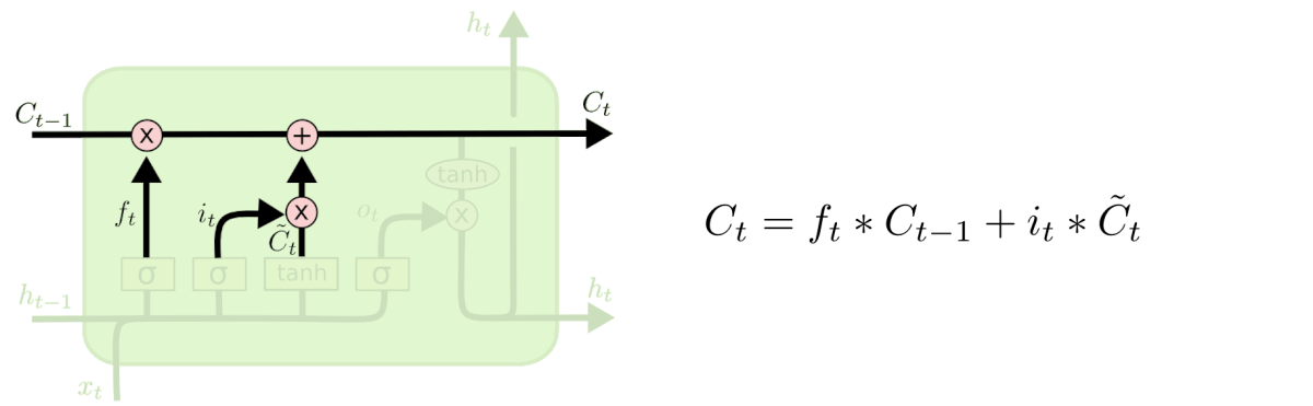
This step is why LSTMs remember. Because the new state is the old state times ft plus something, the gradient flowing back from Ct to Ct−1 is multiplied mainly by ft. When the forget gate is close to 1, the gradient passes through many steps almost without shrinking. Hochreiter and Schmidhuber called this path the constant error carousel.
4. Output gate: what to output
Finally, the LSTM decides what to output. The output is a filtered version of the cell state. A sigmoid layer, the output gate ot, decides which parts of the cell state to output; the cell state goes through tanh to push values between −1 and 1 and is multiplied by the output gate. Having just seen a subject, the language model might output information relevant to the verb that is likely to follow, such as whether the subject is singular or plural.
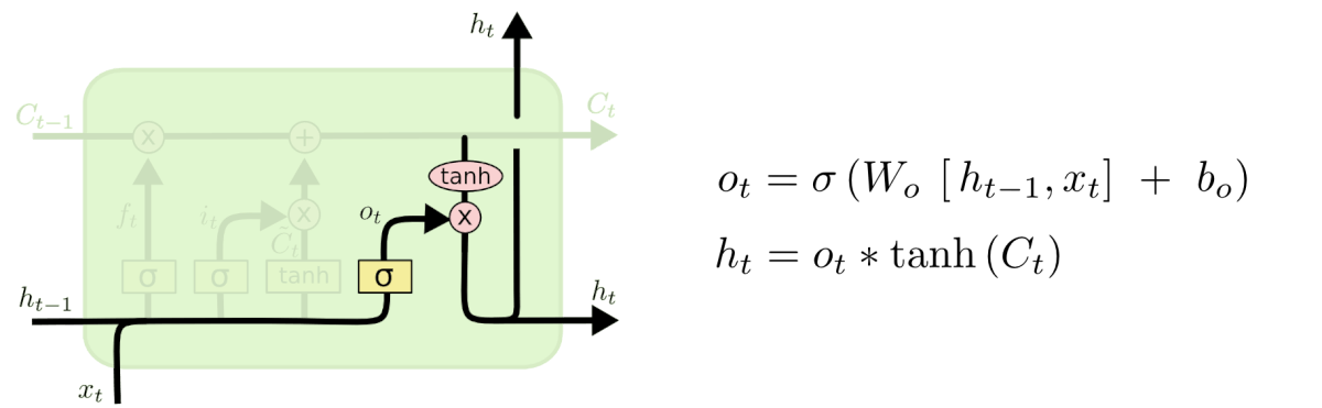
LSTM Equations and a Cell from Scratch
Here are all the steps together. σ is the sigmoid function, [ht−1, xt] is the concatenation of the previous hidden state and the input, and · between vectors is element-wise multiplication:
ft = σ(Wf [ht−1, xt] + bf) forget gate
it = σ(Wi [ht−1, xt] + bi) input gate
C̃t = tanh(WC [ht−1, xt] + bC) candidate values
Ct = ft · Ct−1 + it · C̃t new cell state
ot = σ(Wo [ht−1, xt] + bo) output gate
ht = ot · tanh(Ct) new hidden state
The four layers have the same shape, so an LSTM with input size n and hidden size m has 4 · (m · (n + m) + m) parameters, four times as many as a plain RNN of the same size. The code below implements one LSTM step with these equations and checks that it gives exactly the same result as PyTorch’s nn.LSTMCell:
import torch
import torch.nn as nn

torch.manual_seed(0)
cell = nn.LSTMCell(input_size=3, hidden_size=4)

def lstm_step(x, h, c):
    # PyTorch stacks the weights of the four layers in the order: input, forget, candidate, output
    z = x @ cell.weight_ih.T + cell.bias_ih + h @ cell.weight_hh.T + cell.bias_hh
    i, f, g, o = z.chunk(4, dim=1)
    i, f, g, o = torch.sigmoid(i), torch.sigmoid(f), torch.tanh(g), torch.sigmoid(o)
    c = f * c + i * g            # forget part of the old memory, add scaled new candidates
    h = o * torch.tanh(c)        # output a filtered version of the cell state
    return h, c

x = torch.randn(2, 3)                            # a batch of 2 inputs with 3 features
h, c = torch.zeros(2, 4), torch.zeros(2, 4)      # initial hidden and cell states
h_ours, c_ours = lstm_step(x, h, c)
h_torch, c_torch = cell(x, (h, c))
print("same h:", torch.allclose(h_ours, h_torch, atol=1e-6))
print("same c:", torch.allclose(c_ours, c_torch, atol=1e-6))
print("parameters:", sum(p.numel() for p in cell.parameters()))
same h: True
same c: True
parameters: 144That is 4 · (4 · (3 + 4) + 4) = 128 weights and biases plus 16 more, because PyTorch keeps two bias vectors, one for the input and one for the hidden state, where the equations above have one. In a full nn.LSTM layer the same step simply runs in a loop over the sequence.
Experiment: LSTM vs RNN on Long Sequences
To see the difference between an LSTM and a plain RNN, give both a task that needs memory. Each sequence starts with one of four signal symbols, followed by random noise symbols. After reading the whole sequence, the network must say which signal it started with, so it has to keep one piece of information for the entire length and ignore everything else. We train a plain RNN and an LSTM with the same hidden size on sequences of different lengths:
import torch
import torch.nn as nn

def make_batch(n, length):
    # Each sequence starts with a signal symbol 0-3 followed by random noise symbols 4-7.
    # After reading the whole sequence, the model must say which signal it started with.
    x = torch.randint(4, 8, (n, length))
    y = torch.randint(0, 4, (n,))
    x[:, 0] = y
    return nn.functional.one_hot(x, 8).float(), y

class Classifier(nn.Module):
    def __init__(self, cell, hidden=32):
        super().__init__()
        self.rnn = cell(input_size=8, hidden_size=hidden, batch_first=True)
        self.head = nn.Linear(hidden, 4)

    def forward(self, x):
        out, _ = self.rnn(x)
        return self.head(out[:, -1])             # classify from the state after the last step

def train(cell, length, forget_bias=None, steps=2000, seed=0):
    torch.manual_seed(seed)
    model = Classifier(cell)
    if forget_bias is not None:                  # PyTorch gate order: input, forget, candidate, output
        h = model.rnn.hidden_size
        with torch.no_grad():
            model.rnn.bias_ih_l0[h:2 * h].fill_(forget_bias)
            model.rnn.bias_hh_l0[h:2 * h].fill_(0.0)
    opt = torch.optim.Adam(model.parameters(), lr=3e-3)
    for _ in range(steps):
        x, y = make_batch(64, length)
        loss = nn.functional.cross_entropy(model(x), y)
        opt.zero_grad()
        loss.backward()
        opt.step()
    x, y = make_batch(2000, length)
    with torch.no_grad():
        return (model(x).argmax(1) == y).float().mean().item()

for length in (20, 50, 100):
    rnn = train(nn.RNN, length)
    lstm = train(nn.LSTM, length)
    lstm_fb = train(nn.LSTM, length, forget_bias=3.0)
    print(f"length {length:3d}: RNN {rnn:.2f} | LSTM, default init {lstm:.2f} | LSTM, forget bias 3 {lstm_fb:.2f}")
length 20: RNN 1.00 | LSTM, default init 0.74 | LSTM, forget bias 3 1.00
length 50: RNN 0.25 | LSTM, default init 0.24 | LSTM, forget bias 3 1.00
length 100: RNN 0.26 | LSTM, default init 0.26 | LSTM, forget bias 3 1.00With 20 steps the plain RNN solves the task. With 50 and 100 steps it scores 25%, which is random guessing among four signals: the vanishing gradient problem in action, the network never learns that the first symbol matters.
The surprise is the LSTM with PyTorch’s default initialization: it does no better than the RNN and does not fully solve the task even at 20 steps. The reason is the forget gate. PyTorch initializes all biases with small random values close to zero, so the forget gate starts at about σ(0) = 0.5 and the cell keeps only half of its contents at every step. After 50 steps, 0.550 ≈ 10−15 of the signal is left, and the gradient vanishes just as it does in a plain RNN. Setting the forget gate bias to 3 makes the gate start almost open, at σ(3) ≈ 0.95. The signal and its gradient now survive long enough for training to discover the task and push the gate even closer to 1, and the LSTM is 100% accurate on sequences of 100 steps.
Repeating the experiment with three random seeds and more lengths gives the same picture:
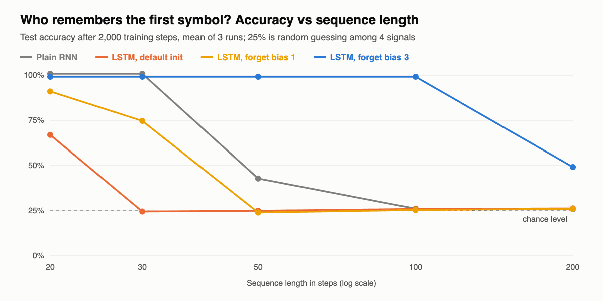
The plain RNN handles up to about 30 steps. The LSTM with default initialization fails beyond 20, and a forget bias of 1 helps only a little. With a forget bias of 3, the LSTM learns every length up to 100 steps in all runs; at 200 steps only one run in three learned the task within 2,000 training steps, so even LSTMs need more training as the gap grows. The practical lesson: an LSTM’s ability to remember depends on its forget gate staying open. Keras adds 1 to the forget gate bias by default (unit_forget_bias=True), while PyTorch does not, so for long sequences it is worth initializing it yourself.
LSTM Variants: Peepholes, Coupled Gates and GRU
What we have described is the standard LSTM, but almost every paper uses a slightly different version. The differences are minor, but some are worth knowing.
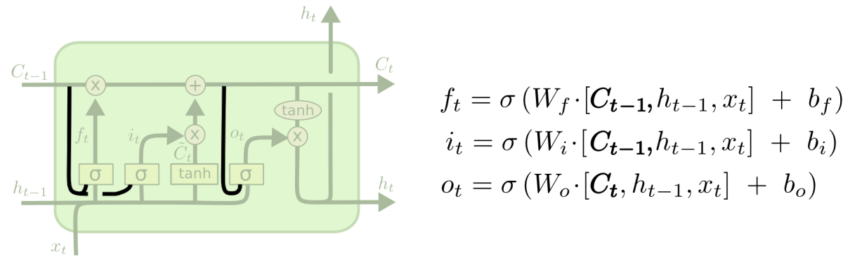
Peephole connections, introduced by Gers and Schmidhuber in 2000, let the gate layers look at the cell state. Some versions give peepholes to all gates, others to only some of them:
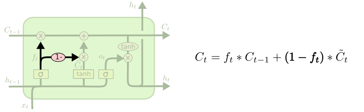
Coupled forget and input gates make the two decisions together: the LSTM forgets only when it is going to write something new in its place, and writes new values only to the components it forgets:
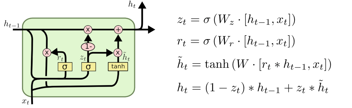
The most popular variant is the gated recurrent unit (GRU), introduced by Kyunghyun Cho and colleagues in 2014. It combines the forget and input gates into a single update gate, merges the cell state and the hidden state, and adds a reset gate. The result is simpler than an LSTM and has fewer parameters:
| LSTM | GRU | |
|---|---|---|
| Gates | Forget, input, output | Update, reset |
| States | Cell state and hidden state | Hidden state only |
| Parameters per layer | 4 sets of weights | 3 sets of weights, about 25% fewer |
| Speed | Slower | Faster to train and run |
| Accuracy | Slightly better on some long or complex sequences | Similar on most tasks, sometimes better on small datasets |
Which variant is best? In “LSTM: A Search Space Odyssey” (2015), Klaus Greff and co-authors compared eight popular variants on speech, handwriting and music tasks and found that none was significantly better than the standard LSTM; the forget gate and the output activation were the most important parts. Rafal Jozefowicz and colleagues at Google tested more than ten thousand recurrent architectures the same year and found a few that beat the LSTM on some tasks, but also that adding a bias of 1 to the LSTM forget gate closed most of the gap with the GRU, which matches the experiment above.
Two other common designs are stacked LSTMs, several LSTM layers on top of each other, each reading the hidden states of the one below, and bidirectional LSTMs, which run one LSTM forward and one backward over the sequence and concatenate their states, so every position sees both past and future context. Bidirectional LSTMs were widely used for speech recognition, named entity recognition and tagging, where the whole sequence is available at once. CNN-LSTM models put a convolutional network in front of an LSTM to extract features from each video frame or image before modeling the sequence.
LSTM for Time Series Forecasting in PyTorch
Time series forecasting is one of the most common uses of LSTMs today. The model below reads a window of the last 48 values of a noisy series with two seasonal cycles and predicts the next value. It is trained on the first 80% of the series and tested on the last 20%, which it has never seen:
import math
import torch
import torch.nn as nn

torch.manual_seed(0)
torch.set_num_threads(1)
# A synthetic time series: two seasonal cycles (periods 50 and 12 steps) plus noise
t = torch.arange(1500, dtype=torch.float32)
series = torch.sin(2 * math.pi * t / 50) + 0.5 * torch.sin(2 * math.pi * t / 12) + 0.1 * torch.randn(1500)

window = 48                                           # look at the last 48 values ...
X = series.unfold(0, window, 1)[:-1].unsqueeze(-1)    # ... shape (samples, 48 steps, 1 feature)
y = series[window:]                                   # ... to predict the next value
split = int(0.8 * len(X))                             # first 80% for training, last 20% for testing
X_train, y_train, X_test, y_test = X[:split], y[:split], X[split:], y[split:]

class Forecaster(nn.Module):
    def __init__(self):
        super().__init__()
        self.lstm = nn.LSTM(input_size=1, hidden_size=32, batch_first=True)
        self.head = nn.Linear(32, 1)

    def forward(self, x):
        out, (h, c) = self.lstm(x)                    # out: hidden state at every step
        return self.head(out[:, -1]).squeeze(-1)      # forecast from the last hidden state

model = Forecaster()
opt = torch.optim.Adam(model.parameters(), lr=1e-2)
for epoch in range(1, 31):
    for idx in torch.randperm(split).split(64):
        loss = nn.functional.mse_loss(model(X_train[idx]), y_train[idx])
        opt.zero_grad()
        loss.backward()
        opt.step()
    if epoch % 10 == 0:
        print(f"epoch {epoch}: train MSE {loss.item():.4f}")

with torch.no_grad():
    lstm_mae = (model(X_test) - y_test).abs().mean().item()
naive_mae = (X_test[:, -1, 0] - y_test).abs().mean().item()   # forecast = last observed value
print(f"test MAE: LSTM {lstm_mae:.3f}, naive last value {naive_mae:.3f}, noise level {0.1 * math.sqrt(2 / math.pi):.3f}")
epoch 10: train MSE 0.0432
epoch 20: train MSE 0.0232
epoch 30: train MSE 0.0228
test MAE: LSTM 0.101, naive last value 0.206, noise level 0.080The LSTM’s mean absolute error on the test data is half that of the naive forecast, which simply repeats the last value, and close to 0.080, the error caused by the random noise that no model can predict. On the plot, its forecasts follow both seasonal cycles:
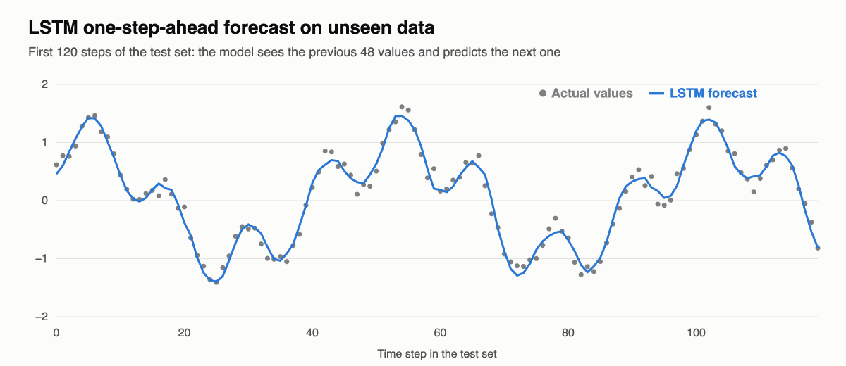
A few practical tips for real data: scale the inputs, for example to zero mean and unit variance; split the data by time, never randomly, so the model is never trained on data from after the period it is tested on; always compare with simple baselines such as the last value, a seasonal naive forecast or linear regression on lagged values; and for tabular features try gradient boosting too, which often wins on business data. LSTMs shine when the series is long, the patterns are non-linear and there are many related series to learn from.
LSTM vs Transformer
When Olah wrote his explanation in 2015, the common opinion among researchers was that the next step after LSTMs would be attention: letting the network look back at any part of the input instead of squeezing everything into one state vector. That is what happened. Attention was first added to LSTM encoder-decoder models for translation and image captioning, and in 2017 the Transformer removed recurrence altogether.
| LSTM | Transformer | |
|---|---|---|
| Processing | Sequential: one step after another | Parallel over all positions |
| Long-range context | Compressed into a fixed-size state | Direct attention to every earlier token |
| Training speed on GPUs | Slow for long sequences | Fast, scales to huge datasets |
| Memory and compute per step at inference | Constant | Grows with context length |
| Data needed | Works with small datasets | Needs a lot of data or pretraining |
| Typical use today | Time series, on-device and streaming models, small sequential tasks | Language models, translation, vision, speech |
Because Transformers can be trained in parallel on enormous datasets, they replaced LSTMs in language modeling, translation and most of speech recognition. But the advantages of recurrence, constant memory per step and natural streaming, never went away, and since 2023 recurrent ideas have come back. State space models such as Mamba and linear recurrent networks such as RWKV process sequences step by step while training in parallel. In 2024 Sepp Hochreiter’s team presented xLSTM, which adds exponential gating and a matrix memory to the LSTM and reported results competitive with Transformers and state space models of similar size on language modeling.
Applications of LSTM
- Time series forecasting: demand, energy load, traffic, weather, financial and sensor data.
- Speech recognition and synthesis: LSTM acoustic models powered voice assistants in the 2010s and are still used in compact on-device models.
- Language and text: machine translation before Transformers, text classification, sentiment analysis, named entity recognition, keyboard next-word prediction.
- Handwriting recognition and text generation, including Alex Graves’s well-known handwriting synthesis model.
- Video and activity recognition with CNN-LSTM models.
- Anomaly detection in logs, network traffic and industrial equipment.
- Reinforcement learning agents that need memory, such as OpenAI Five for Dota 2 and AlphaStar for StarCraft II.
FAQ
What is the full form of LSTM?
LSTM stands for long short-term memory. The name means that the network keeps a short-term memory, its internal state, for a long time.
What is an LSTM in simple terms?
It is a recurrent neural network with a memory cell and three gates. At each step of a sequence, the gates decide what to forget from memory, what new information to store and what to output, which lets the network remember important information over hundreds of steps.
What is the difference between an RNN and an LSTM?
An LSTM is a kind of RNN. A plain RNN overwrites its hidden state at every step with a single tanh layer, so information and gradients fade within a few dozen steps. An LSTM adds a cell state that is updated by addition and controlled by gates, so it can keep information much longer.
What are the gates of an LSTM?
The forget gate decides what to remove from the cell state, the input gate decides which new values to write, and the output gate decides which parts of the cell state become the output. Each gate is a sigmoid layer whose outputs between 0 and 1 scale the information element by element.
Is LSTM better than GRU?
Neither is better in general. GRUs are simpler and faster and perform about as well on most tasks; LSTMs are sometimes slightly better on long or complex sequences. It is common to try both.
Is LSTM still used in 2026?
Yes, though no longer for large language models. LSTMs remain popular for time series forecasting, streaming and on-device speech, small datasets and as components of larger systems, and new recurrent designs such as xLSTM build directly on them.
Is LSTM supervised or unsupervised?
An LSTM is an architecture, not a learning method. It is usually trained with supervised learning, for example to classify sequences or predict the next value, but it can also be trained in self-supervised or reinforcement learning settings. See our guide to supervised, unsupervised and reinforcement learning.
See also: our guides to backpropagation, which explains how gradients flow through networks, and to activation functions, including the sigmoid and tanh used in LSTM gates.