An autoencoder is a neural network that learns to copy its input to its output through a narrow bottleneck. Because it cannot simply pass every number through, it has to learn a compact summary of the data, a code in the so-called latent space, and a way to rebuild the original from it. This simple trick turns out to be useful for compression, denoising, anomaly detection and feature learning, and it is a building block of modern AI: image generators such as Stable Diffusion work in the latent space of an autoencoder, and sparse autoencoders are one of the main tools researchers use to look inside large language models.
This guide explains what an autoencoder is, how its architecture works, the main types of autoencoders (undercomplete, deep, convolutional, sparse, denoising, variational and masked) and where they are used. In a hands-on PyTorch experiment we compare an autoencoder with PCA, remove noise from images and use an autoencoder to detect clothing it has never seen.
Key takeaways
- An autoencoder has two parts: an encoder that compresses the input into a short code and a decoder that reconstructs the input from that code. It is trained to make the reconstruction as close to the input as possible.
- It needs no labels: the input is its own target, so autoencoders are a form of unsupervised (self-supervised) learning.
- The bottleneck or a regulariser stops it from learning a useless identity copy and forces it to capture the structure of the data.
- Types: undercomplete, deep, convolutional, sparse, denoising, contractive, variational (VAE) and masked autoencoders.
- In our experiment on Fashion-MNIST, an autoencoder that squeezed 784 pixels into 8 numbers reconstructed images with 44% less error than PCA, raised image quality from 12.8 to 19.0 dB PSNR when removing noise, and spotted unseen types of clothing with a ROC AUC of 0.87 to 0.94.
What is an autoencoder?
An autoencoder (AE) is a type of neural network trained to reproduce its input. A photo goes in, and the network tries to output the same photo. What makes this non-trivial is that the data has to pass through a layer that is much smaller than the input, or through a layer that is constrained in some other way. To succeed, the network must discover which features of the data matter and store only those.
Autoencoders learn without labels: the training target is the input itself. That makes them an example of unsupervised learning, or more precisely self-supervised learning, where the data provides its own supervision. The idea goes back to the 1980s; in 2006 Geoffrey Hinton and Ruslan Salakhutdinov showed in Science that deep autoencoders compress images and documents far better than principal component analysis (PCA), one of the results that started the deep learning revival.
Autoencoder architecture
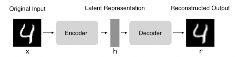
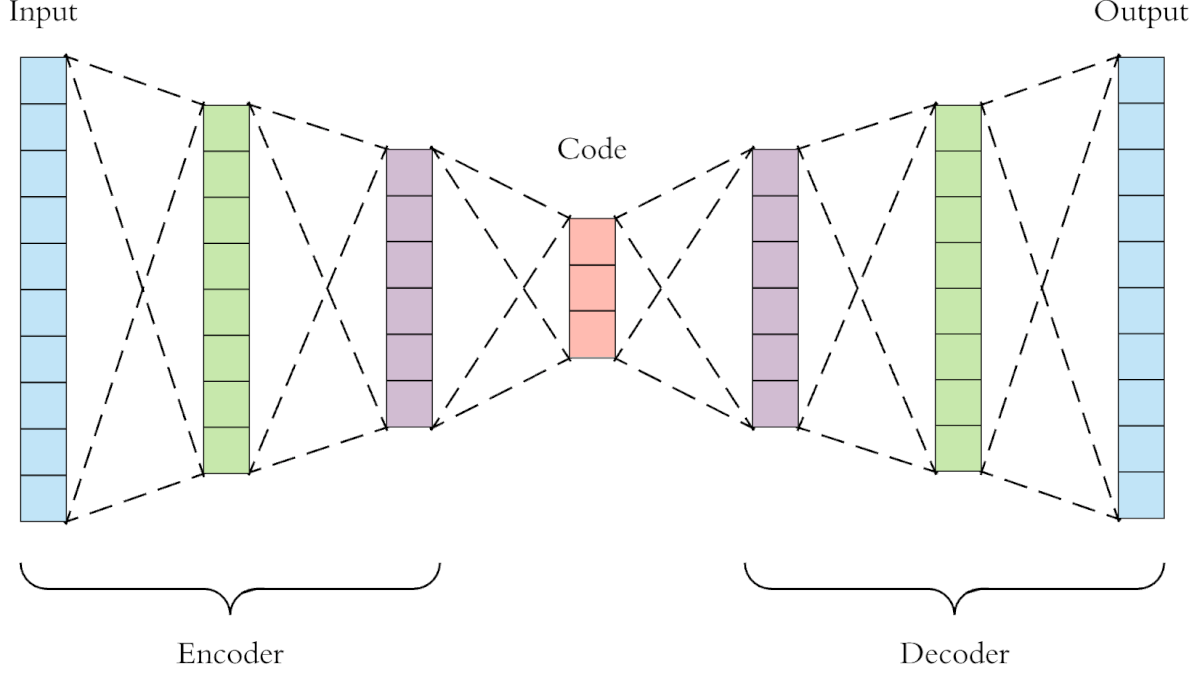
Every autoencoder has three parts:
- Encoder h = f(x): a network that maps the input x to a code h. For images it is usually a stack of fully connected or convolutional layers that get smaller towards the middle.
- Code, or bottleneck: the compressed representation h, a point in the latent space. Its size is the most important design choice: in our experiment a 784-pixel image is squeezed into 2 to 64 numbers.
- Decoder r = g(h): a network, usually a mirror image of the encoder, that maps the code back to a reconstruction r with the same shape as the input.
The whole model computes r = g(f(x)), and training minimises a reconstruction loss that measures how different r is from x: the mean squared error for real values, or binary cross-entropy for pixels between 0 and 1. The weights are updated with backpropagation and gradient descent, exactly like any other network. The input and output layers always have the same size.
After training, the two halves can be used separately. The encoder alone turns data into compact features for search, clustering or visualisation; the decoder alone turns codes into data, which is the basis of generative models.
Why copy the input to the output?
An autoencoder that copies its input perfectly would be useless. If the code is as large as the input, or larger, even a linear network can learn the identity function and pass every pixel straight through without learning anything about the data. The value lies in the code h, and the code becomes useful only when the network is prevented from copying. There are two ways to do that:
- Limit the capacity of the code. An undercomplete autoencoder has a code smaller than the input, so it has to keep the most important information and drop the rest.
- Add a different constraint. Regularised autoencoders may have a large code but are trained with an extra requirement: most code units must be zero (sparse), the input is corrupted with noise that must be removed (denoising), or the code must be insensitive to small changes in the input (contractive).
In both cases the network learns the structure of the data distribution: which pixel patterns appear together in shirts, which in shoes. That knowledge is what makes autoencoders useful for denoising and detecting anomalies. It also explains their main limitation as compressors: an autoencoder works only on data similar to what it was trained on. An autoencoder trained on clothing photos cannot compress a landscape photo, while JPEG works on any image.
Types of autoencoders
Undercomplete (vanilla) autoencoder
The simplest form: an input layer, one hidden layer that is smaller than the input, and an output layer. With linear activations and a squared error loss it learns the same subspace as PCA; with non-linear activations it can capture curved structure that PCA misses.
Deep (stacked) autoencoder
When one hidden layer is not enough, the encoder and decoder get several layers each, usually symmetric, such as 784 → 256 → 32 → 256 → 784. More layers let the network learn more complex, hierarchical features. In the 2000s deep autoencoders were trained layer by layer (“stacked”) because training deep networks end to end was hard; today they are trained in one go.
Convolutional autoencoder
For images, the fully connected layers are replaced by convolutional layers. The encoder reduces the spatial resolution step by step with strided convolutions or pooling; the decoder increases it again with transposed convolutions or upsampling. Convolutional autoencoders need far fewer weights and preserve local image structure much better.
Sparse autoencoder
A sparse autoencoder may have a code that is larger than the input, but a penalty in the loss, for example the L1 norm of the code activations, forces most code units to be zero for any given input. Each unit then becomes a detector for a specific feature that is present only in some inputs. This property made sparse autoencoders a key tool in AI interpretability: Anthropic used them in 2023 and 2024 to decompose the internal activations of language models, including Claude 3 Sonnet, into millions of human-interpretable features such as “the Golden Gate Bridge” or “code with a security vulnerability”. OpenAI and Google DeepMind published similar work on GPT-4 and on the open Gemma models (Gemma Scope).
Denoising autoencoder
Introduced by Pascal Vincent and colleagues in 2008, a denoising autoencoder receives a corrupted input, for example an image with random noise or missing pixels, and is trained to reconstruct the clean original. It cannot just copy its input, because the input is wrong; it has to learn what clean data looks like. Our experiment below shows how much noise a small denoising autoencoder can remove.
Contractive autoencoder
A contractive autoencoder adds a penalty on how much the code changes when the input changes slightly (the norm of the encoder’s Jacobian). The result is a code that is robust to small variations and captures only the directions in which the data really varies.
Variational autoencoder (VAE)
A variational autoencoder, proposed by Diederik Kingma and Max Welling in 2013, turns the autoencoder into a generative model. The encoder outputs a probability distribution over codes instead of a single point, and an extra loss term keeps that distribution close to a standard normal distribution. As a result, the latent space is smooth and continuous: you can sample a random code, run it through the decoder and get a new, realistic example. VAEs are the reason latent diffusion works: Stable Diffusion and many newer image and video generators first compress images with a VAE (a 512 × 512 colour image becomes a 64 × 64 × 4 latent, 48 times fewer numbers) and run the expensive diffusion process in that latent space.
Masked autoencoder (MAE)
Masked autoencoders, introduced by Kaiming He and colleagues at Meta in 2021, hide a large part of the input, typically 75% of the patches of an image, and train a transformer to reconstruct the missing parts. Solving this puzzle forces the model to understand the content of the image, so the encoder becomes an excellent pretrained backbone for classification and detection. The same idea of predicting hidden parts of the input underlies BERT in language.
Experiment: an autoencoder in PyTorch
We trained small fully connected autoencoders on Fashion-MNIST, an open data set from Zalando Research (MIT licence) with 60,000 training and 10,000 test images of clothing, 28 × 28 grayscale pixels each. The encoder has the shape 784 → 256 → code and the decoder mirrors it. Three tests:
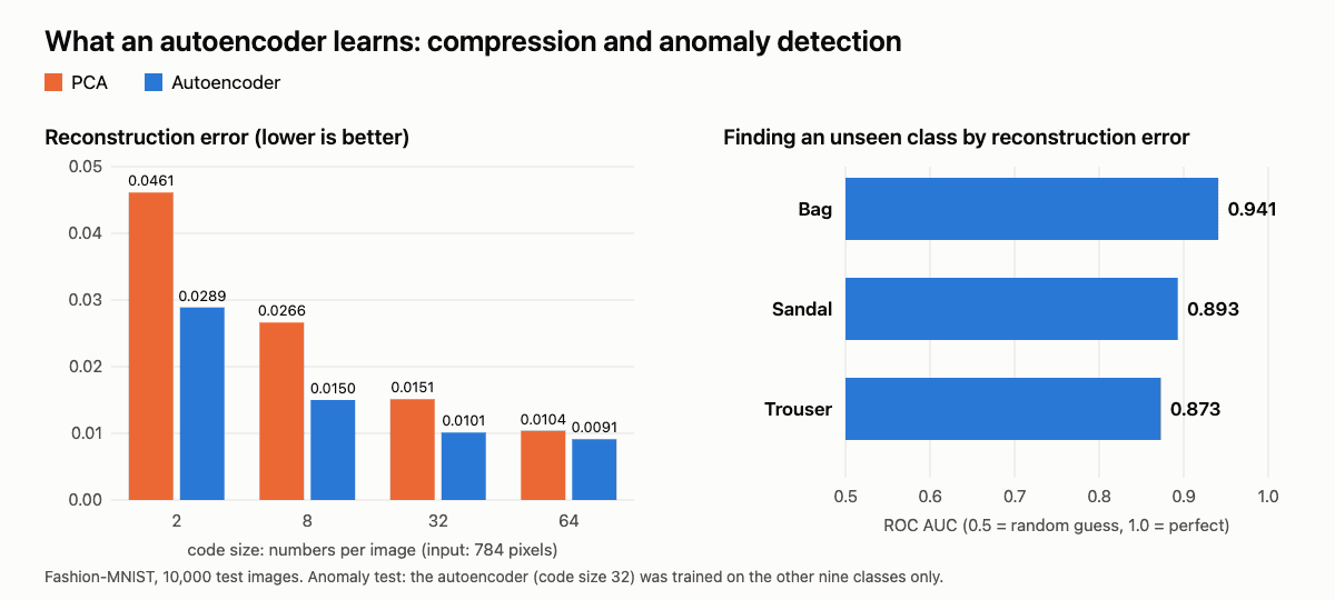
- Compression: an autoencoder against PCA with the same code size, from 2 to 64 numbers per image, measured by the mean squared reconstruction error on the test images.
- Denoising: random noise (standard deviation 0.3) is added to every image; a denoising autoencoder learns to output the clean version.
- Anomaly detection: an autoencoder is trained on nine of the ten classes and must flag the tenth, which it has never seen, by its reconstruction error. We repeated this for bags, trousers and sandals.
The code needs PyTorch, scikit-learn and NumPy. Download the four .gz files from the data/fashion folder of the Fashion-MNIST repository on GitHub into a data folder next to the script. It runs in about five minutes on an ordinary two-core CPU.
import gzip

import numpy as np
import torch
from torch import nn
from sklearn.decomposition import PCA
from sklearn.metrics import roc_auc_score

# Fashion-MNIST: 60,000 training and 10,000 test images of clothes, 28x28 pixels (MIT licence, Zalando Research)
def load(kind):
    with gzip.open(f"data/{kind}-images-idx3-ubyte.gz") as f:
        x = np.frombuffer(f.read(), np.uint8, offset=16).reshape(-1, 784) / 255.0
    with gzip.open(f"data/{kind}-labels-idx1-ubyte.gz") as f:
        y = np.frombuffer(f.read(), np.uint8, offset=8)
    return torch.tensor(x, dtype=torch.float32), y

x_train, y_train = load("train")
x_test, y_test = load("t10k")
torch.manual_seed(0)

class Autoencoder(nn.Module):
    def __init__(self, code_size):
        super().__init__()
        self.encoder = nn.Sequential(nn.Linear(784, 256), nn.ReLU(), nn.Linear(256, code_size))
        self.decoder = nn.Sequential(nn.Linear(code_size, 256), nn.ReLU(), nn.Linear(256, 784), nn.Sigmoid())

    def forward(self, x):
        return self.decoder(self.encoder(x))

def train(model, inputs, targets, epochs=15):
    opt = torch.optim.Adam(model.parameters(), lr=1e-3)
    for epoch in range(epochs):
        for idx in torch.randperm(len(inputs)).split(256):
            loss = nn.functional.mse_loss(model(inputs[idx]), targets[idx])  # reconstruction error
            opt.zero_grad()
            loss.backward()
            opt.step()
    return model.eval()

def mse(a, b):
    return ((a - b) ** 2).mean().item()

# 1. Compression: autoencoder vs PCA with the same code size
for k in [2, 8, 32, 64]:
    pca = PCA(k).fit(x_train.numpy())
    pca_rec = torch.tensor(pca.inverse_transform(pca.transform(x_test.numpy())), dtype=torch.float32)
    ae = train(Autoencoder(k), x_train, x_train)
    with torch.no_grad():
        ae_rec = ae(x_test)
    print(f"code size {k:2d}: 784 numbers -> {k:2d}  PCA error {mse(pca_rec, x_test):.4f}  autoencoder error {mse(ae_rec, x_test):.4f}")

# 2. Denoising: train on noisy inputs, compare the output with the clean image
noisy_train = (x_train + 0.3 * torch.randn_like(x_train)).clamp(0, 1)
noisy_test = (x_test + 0.3 * torch.randn_like(x_test)).clamp(0, 1)
dae = train(Autoencoder(64), noisy_train, x_train)
with torch.no_grad():
    denoised = dae(noisy_test)
psnr = lambda a, b: 10 * np.log10(1 / mse(a, b))
print(f"denoising: noisy image PSNR {psnr(noisy_test, x_test):.1f} dB -> denoised {psnr(denoised, x_test):.1f} dB")

# 3. Anomaly detection: learn only "normal" clothes, then flag images that reconstruct badly
for anomaly, name in [(8, "Bag"), (1, "Trouser"), (5, "Sandal")]:
    ae = train(Autoencoder(32), x_train[y_train != anomaly], x_train[y_train != anomaly])
    with torch.no_grad():
        error = ((ae(x_test) - x_test) ** 2).mean(dim=1).numpy()
    auc = roc_auc_score(y_test == anomaly, error)
    print(f"anomaly '{name}': error on normal {error[y_test != anomaly].mean():.4f}, "
          f"on unseen class {error[y_test == anomaly].mean():.4f}, ROC AUC {auc:.3f}")
code size 2: 784 numbers -> 2 PCA error 0.0461 autoencoder error 0.0289
code size 8: 784 numbers -> 8 PCA error 0.0266 autoencoder error 0.0150
code size 32: 784 numbers -> 32 PCA error 0.0151 autoencoder error 0.0101
code size 64: 784 numbers -> 64 PCA error 0.0104 autoencoder error 0.0091
denoising: noisy image PSNR 12.8 dB -> denoised 19.0 dB
anomaly 'Bag': error on normal 0.0094, on unseen class 0.0264, ROC AUC 0.941
anomaly 'Trouser': error on normal 0.0106, on unseen class 0.0209, ROC AUC 0.873
anomaly 'Sandal': error on normal 0.0097, on unseen class 0.0234, ROC AUC 0.893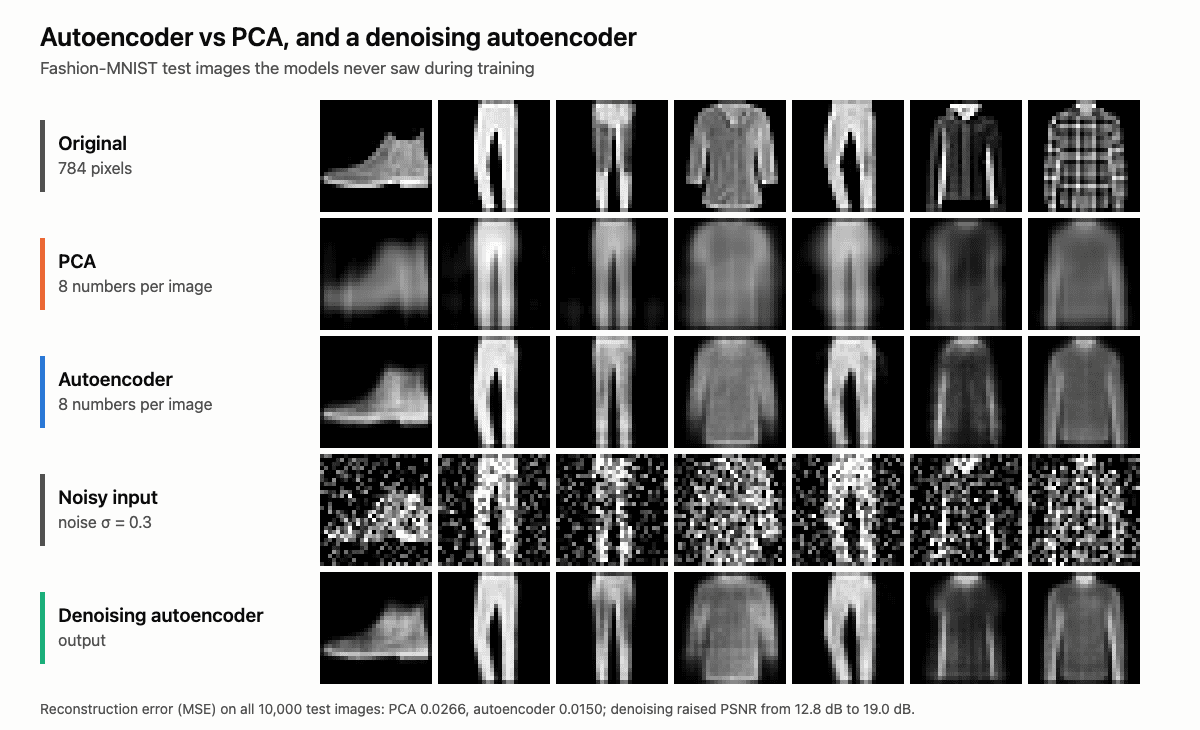
What the results show:
- Non-linear compression beats PCA, especially for small codes. With 8 numbers per image the autoencoder’s error was 0.0150 against 0.0266 for PCA, 44% lower; with 2 numbers it was 37% lower. With 64 numbers the gap shrinks to 13%, because PCA with many components already captures most of the variation. The picture shows the difference: PCA with 8 components gives grey, ghostly shapes, while the autoencoder keeps the outline of a boot or a shirt. Both lose fine details such as prints and checks, the typical blur of autoencoders trained with a squared error.
- Denoising works without ever seeing the noise-free test images. The noisy inputs have a peak signal-to-noise ratio (PSNR) of 12.8 dB; the denoising autoencoder raised it to 19.0 dB, which means it reduced the squared error about four times (each 10 dB is a factor of ten).
- Reconstruction error is a usable anomaly score. The autoencoder rebuilt the unseen class two to three times worse than normal clothing: an average error of 0.0264 for bags against 0.0094 for the nine known classes. Ranking test images by error found bags with a ROC AUC of 0.941 (1.0 is perfect, 0.5 is random guessing), sandals with 0.893 and trousers with 0.873. Trousers were the hardest, probably because their simple vertical shape is easy to approximate from what the network learned on dresses and other long garments.
Everything here used tiny models trained in minutes. Convolutional autoencoders, larger codes for denoising, or a VAE would improve every number, but the pattern stays the same.
Applications
- Dimensionality reduction and visualisation. Encoding data into two or three dimensions to plot it, or into a few dozen dimensions to speed up other algorithms.
- Denoising and restoration. Removing noise from images, audio and sensor signals; denoising ideas also underlie image restoration and super resolution and diffusion models.
- Anomaly detection. Train on normal data only, then flag inputs with a high reconstruction error: fraudulent transactions, defective products on a production line, unusual network traffic or failing machines.
- Feature learning and pretraining. The encoder of a trained autoencoder, especially a masked autoencoder, provides features for classifiers when labelled data is scarce.
- Generative models. VAEs generate new data and provide the latent space for latent diffusion models that create images, video and audio.
- Recommendations. Autoencoders that reconstruct a user’s interaction history, such as Mult-VAE, are strong baselines for recommender systems.
- Interpretability. Sparse autoencoders trained on the activations of a language model reveal the concepts the model represents internally, which helps researchers find and steer behaviours.
- Learned compression. Neural image and audio codecs are built on autoencoders; for audio, codecs such as Google’s SoundStream and Meta’s EnCodec compress speech and music into discrete codes that language-model-style generators then work with.
Autoencoder vs PCA
Principal component analysis finds the linear directions along which the data varies most and projects the data onto them. A linear autoencoder with a squared error loss learns the same subspace. The difference appears with non-linear layers:
| PCA | Autoencoder | |
|---|---|---|
| Mapping | Linear projection | Non-linear, learned by a neural network |
| Training | Exact solution in seconds | Iterative training with gradient descent |
| Small codes | Loses a lot of information | Usually reconstructs much better |
| Interpretability | Components are ordered and orthogonal | Code dimensions have no fixed meaning |
| Data needed | Works with little data | Needs more data to avoid overfitting |
Use PCA as a fast baseline and when the data is small or roughly linear; use an autoencoder when the structure is complex, the data is large, or you need a decoder that generates data.
Limitations
- Domain-specific. An autoencoder compresses well only data similar to its training data.
- Blurry reconstructions. Trained with a squared error, autoencoders average over possibilities and lose fine details; generative models add adversarial or perceptual losses to fix this.
- Risk of trivial solutions. With too large a code or too much capacity, an autoencoder can learn to copy the input without learning useful features.
- Unstructured latent space. A plain autoencoder’s latent space has gaps, so random codes do not decode into realistic data; variational autoencoders solve this.
- Anomaly detection is not perfect. Anomalies that look similar to normal data are reconstructed well and slip through, and a powerful autoencoder can learn to reconstruct some anomalies too; in our experiment trousers were the hardest class to detect.
FAQ
What is an autoencoder in simple terms?
It is a neural network that learns to compress data and then rebuild it. Because the compressed version is small, the network has to learn what is important in the data, and that learned summary can be used for denoising, finding anomalies or generating new data.
Is an autoencoder supervised or unsupervised?
It is trained without labels, so it is usually classed as unsupervised or self-supervised learning: the input serves as its own target.
What is the difference between an autoencoder and a variational autoencoder?
A standard autoencoder maps each input to one point in the latent space and is used mainly for compression and features. A variational autoencoder maps each input to a probability distribution and regularises the latent space, so it can generate new data by sampling random codes.
What is the latent space?
It is the space of codes produced by the encoder. Similar inputs end up close to each other in it, so the latent space captures the structure of the data in far fewer dimensions than the original.
What is the difference between an encoder-decoder model and an autoencoder?
Every autoencoder is an encoder-decoder model, but not every encoder-decoder model is an autoencoder. In translation, for example, a transformer encoder reads a sentence in one language and the decoder writes a different sentence in another language. In an autoencoder the decoder’s target is the input itself.
Can autoencoders be used for anomaly detection?
Yes, this is one of their most common uses. An autoencoder trained only on normal data reconstructs normal inputs well and unusual inputs badly, so a high reconstruction error flags a likely anomaly. In our experiment this found unseen bags, sandals and trousers with a ROC AUC between 0.87 and 0.94.