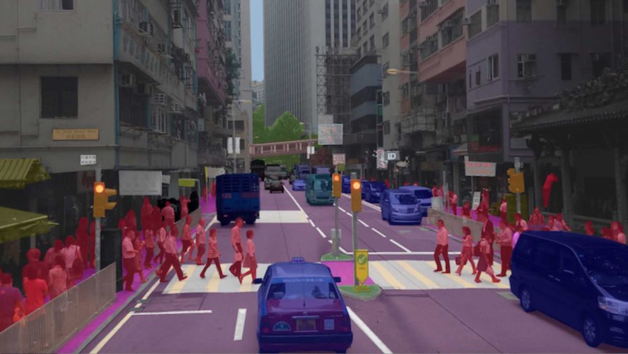
Semantic segmentation is the computer vision task of assigning a class label to every pixel of an image: this pixel is road, that one is a pedestrian, those are sky. Where image classification answers “what is in the picture?” and object detection answers “where are the objects?”, semantic segmentation draws their exact outlines. It is what lets a self-driving car see where the drivable road ends, a radiologist measure a tumour, or a video call blur the background behind you.
This guide explains how semantic segmentation works: how it differs from instance and panoptic segmentation, how encoder-decoder networks such as FCN and U-Net turn an image into a pixel map, which loss functions and metrics are used, and where foundation models such as Segment Anything fit in. We also trained four segmenters on the CamVid street-scene data set, from a pixel-by-pixel random forest to a U-Net, and measured what each design choice adds. The PyTorch code runs on a laptop CPU.
Key takeaways
- Semantic segmentation classifies every pixel. It does not separate individual objects: two cars side by side become one “car” region. Instance segmentation separates them; panoptic segmentation does both.
- Most models are encoder-decoders. The encoder shrinks the image to capture context; the decoder enlarges it back to full resolution. U-Net’s skip connections pass fine detail from encoder to decoder.
- Mean IoU is the main metric, not pixel accuracy: on street scenes, a model can label 80% of pixels correctly and still miss almost every pole, sign and cyclist.
- In our test on CamVid, a U-Net trained from scratch on 468 images reached 0.48 mean IoU, almost twice the 0.25 of a random forest that classifies pixels one by one. Skip connections alone added 0.09 mean IoU, mostly on thin and small objects.
- In 2026, foundation models dominate: Meta’s SAM 3 segments any object described by a short text prompt, and pretrained backbones such as DINOv3 make strong segmenters from few labels.
What is semantic segmentation?
Semantic segmentation takes an image of H × W pixels and returns a segmentation mask of the same size, in which every pixel holds the number of a class from a fixed list, for example 0 = sky, 1 = building, 3 = road. Shown in colour, the mask looks like a colouring book filled in by the model.
It is the most detailed of the three classic computer vision tasks:
- Image classification gives one label for the whole image: “a street”.
- Object detection draws a box around each object and labels it: “car, at these coordinates”. Boxes are cheap but crude; a box around a cyclist also contains road and sky.
- Semantic segmentation labels each pixel, so it captures exact shapes and areas, and it also covers “stuff” without a clear shape, such as road, grass, sky or water, which detection handles poorly.
Technically, a segmentation network is a classifier applied to every pixel at once. For each pixel it outputs a vector of scores, one per class, and the predicted label is the class with the highest score. The difficulty is that the label of a pixel depends on its context: a grey pixel may be road, building or sky, and only the surrounding area tells which. A good model must see both the big picture and the fine detail at the boundaries.
Semantic vs instance vs panoptic segmentation
Segmentation comes in three flavours, which differ in whether they separate individual objects:
| Semantic segmentation | Instance segmentation | Panoptic segmentation | |
|---|---|---|---|
| Labels every pixel? | Yes | No, only countable objects | Yes |
| Separates objects of one class? | No: three cars form one “car” region | Yes: car 1, car 2, car 3 | Yes, for objects (“things”) |
| Handles road, sky, grass (“stuff”)? | Yes | No | Yes |
| Typical models | FCN, U-Net, DeepLab, SegFormer | Mask R-CNN, YOLO segmentation models, SAM | Panoptic FPN, Mask2Former, OneFormer |
| Use when | You need areas and boundaries: road, organ, land cover | You need to count or track objects | You need a complete scene description |
Instance segmentation usually extends an object detector with a mask for each detected box, as Mask R-CNN does. Panoptic segmentation, introduced in 2018, combines both: every pixel gets a class, and pixels of countable objects also get an instance ID. Modern architectures such as Mask2Former handle all three tasks with one design.
How semantic segmentation networks work
An ordinary convolutional neural network for classification gradually shrinks the image: each pooling or strided convolution halves the resolution, so that deep layers see large areas and recognise objects, and a final fully connected layer outputs one label. Segmentation needs the opposite at the end: a prediction for every pixel at full resolution.
Fully convolutional networks
The breakthrough came in 2015 with fully convolutional networks (FCN) by Long, Shelhamer and Darrell. They replaced the fully connected layers of a classification network with convolutions, so the network outputs a coarse map of class scores instead of a single vector, and then upsampled this map back to the size of the input. Because it has no fully connected layers, an FCN accepts images of any size. Its weakness is blurry boundaries: the coarse map, 32 times smaller than the image in the original FCN-32s, loses the fine detail.
Encoder-decoder architecture and U-Net
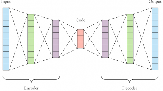
Most segmentation networks today follow an encoder-decoder design. The encoder is a classification-style network that reduces resolution and increases the number of feature channels, learning what is in the image. The decoder increases the resolution step by step with upsampling or transposed convolutions, recovering where things are.
U-Net, published the same year by Ronneberger, Fischer and Brox for biomedical images, added skip connections: at each resolution, the decoder receives a copy of the encoder’s feature maps, which still contain sharp edges and fine texture. The decoder thus combines deep, semantic features with shallow, precise ones. Drawn as a diagram, the contracting and expanding paths form a “U”, hence the name. U-Net works well even with a few dozen training images, and it remains the default architecture in medical imaging and it was the backbone of the first diffusion image generators, such as Stable Diffusion 1 and 2.
Dilated convolutions and multi-scale context
Another way to keep resolution is the dilated (atrous) convolution, which spaces out the kernel weights so that a 3 × 3 kernel covers a 5 × 5 or 9 × 9 area without extra parameters or downsampling. Google’s DeepLab family uses dilated convolutions and an atrous spatial pyramid pooling module that looks at the image at several dilation rates in parallel, capturing small and large objects at once. PSPNet (2017) does something similar with a pyramid of pooling layers. Before deep networks learned enough context on their own, many models also refined their output with a conditional random field (CRF), which encourages neighbouring pixels with similar colours to share a label.
Transformers and mask classification
Since 2021, vision transformers have replaced convolutional encoders in many top models: self-attention lets every image patch interact with every other one from the first layer, so global context is available everywhere. SegFormer (2021) paired an efficient hierarchical transformer encoder with a lightweight decoder. Mask2Former (2022) changed the formulation itself: instead of classifying each pixel, it predicts a set of masks and a class for each mask, which handles semantic, instance and panoptic segmentation with one architecture.
Semantic segmentation models: from FCN to SAM 3
| Year | Model | Key idea |
|---|---|---|
| 2015 | FCN | Classification network turned fully convolutional, outputs a per-pixel map |
| 2015 | U-Net, SegNet | Symmetric encoder-decoder; skip connections (U-Net) or pooling indices (SegNet) restore detail |
| 2015–2018 | DeepLab v1–v3+ | Dilated convolutions, atrous spatial pyramid pooling, CRF refinement in early versions |
| 2017 | PSPNet | Pyramid pooling for global scene context |
| 2017 | Mask R-CNN | Instance segmentation: a mask for every detected object |
| 2021 | SegFormer | Efficient transformer encoder with a simple decoder |
| 2022 | Mask2Former | Mask classification: one architecture for semantic, instance and panoptic segmentation |
| 2023 | Segment Anything (SAM) | Promptable segmentation: click a point or draw a box, get a mask for any object; trained on 1.1 billion masks |
| 2024 | SAM 2 | Extends promptable segmentation to video with object tracking |
| 2025 | DINOv3, SAM 3 | Self-supervised backbone with strong dense features; SAM 3 segments all instances of a concept given a short text or an example image |
Segment Anything deserves a note. The original SAM, released by Meta in April 2023 together with the SA-1B data set of 11 million images and 1.1 billion masks, segments whatever you point at, but it does not know what the object is. SAM 3, released in November 2025, adds promptable concept segmentation: given a phrase such as “yellow school bus” or an example image, it finds, segments and tracks every matching object in images and video. Meta reports that it roughly doubles the accuracy of earlier systems on its SA-Co benchmark and processes an image with more than 100 objects in 30 milliseconds on an H200 GPU. In practice, such open-vocabulary models are increasingly used to label training data for smaller, specialised segmenters, and directly when the classes are not known in advance. Domain versions exist too, for example MedSAM2 for 3D medical images and video.
Loss functions and class imbalance
Training compares the predicted score maps with the ground-truth mask pixel by pixel. The standard loss is pixel-wise cross-entropy: softmax turns each pixel’s scores into class probabilities, and the loss is the average negative log-probability of the true class over all pixels. Pixels marked “void” or “unlabelled” are simply ignored.
The trouble is class imbalance. In street scenes, road, buildings and sky cover most of the image, while poles, signs and cyclists occupy a few percent or less: in CamVid’s training images, road takes 32% of the pixels and bicyclists 0.3%. A network trained with plain cross-entropy can reach a low loss while ignoring small classes. Common remedies:
- Class weights. Multiply each pixel’s loss by a weight that is larger for rare classes. SegNet used median frequency balancing: the weight of a class is the median class frequency divided by its own frequency.
- Dice loss. Based on the Dice coefficient (see below), it measures overlap per class and is less dominated by large classes. It is very popular in medical imaging, where the object of interest, such as a lesion, may cover 1% of the image. Many models combine Dice and cross-entropy.
- Focal loss. Down-weights pixels that are already classified confidently, so training focuses on hard pixels.
Metrics: pixel accuracy, IoU and Dice
- Pixel accuracy is the share of correctly labelled pixels. It is easy to understand but misleading: a model that labels everything as road, building or sky can score high while missing every small object.
- Intersection over union (IoU), also called the Jaccard index, is computed for each class: the number of pixels that both the prediction and the ground truth assign to the class (intersection), divided by the number of pixels that either assigns to it (union). IoU = TP / (TP + FP + FN). It is 1 for a perfect match and 0 for no overlap.
- Mean IoU (mIoU) averages IoU over all classes, so a small class counts as much as a large one. It is the standard metric of segmentation benchmarks.
- Dice coefficient, or F1 score for masks: 2 × TP / (2 × TP + FP + FN). It is closely related to IoU (Dice = 2 IoU / (1 + IoU)) and is the usual metric in medical imaging.
Our experiment below shows why the difference matters: the gap between models in pixel accuracy is much smaller than the gap in mean IoU.
Semantic segmentation datasets
| Dataset | Content | Size | Classes |
|---|---|---|---|
| PASCAL VOC 2012 | Everyday objects | About 2,900 images with segmentation masks (about 10,600 with additional annotations) | 20 + background |
| Cityscapes | Street scenes from 50 cities | 5,000 finely annotated images, 20,000 coarsely annotated | 19 used for evaluation |
| ADE20K | Indoor and outdoor scenes | About 20,000 training and 2,000 validation images | 150 in the scene parsing benchmark |
| COCO-Stuff | COCO photos with “stuff” classes added | 164,000 images | 171 (80 things, 91 stuff) |
| CamVid | Video frames from a car in Cambridge | 701 labelled frames | 11 in the common setup |
Medical imaging has its own benchmarks, such as the Medical Segmentation Decathlon, with ten tasks from brain tumours to the spleen, and satellite imagery has land-cover data sets such as LoveDA and DeepGlobe.
Experiment: four segmenters on CamVid
To see what each idea contributes, we trained four segmenters on CamVid, the street-scene data set used in the SegNet paper: 367 training, 101 validation and 233 test frames from a car driving around Cambridge, UK, labelled with 11 classes plus “void”. We used the version from the SegNet tutorial repository on GitHub and reduced the images from 480 × 360 to 192 × 144 pixels so that everything trains on a CPU:
- Random forest on colour and position. A classic baseline: each pixel is classified on its own from five numbers, its red, green and blue values and its row and column, with no knowledge of neighbouring pixels.
- FCN-style encoder-decoder without skip connections: the encoder shrinks the image 16 times, the decoder enlarges it back.
- U-Net: the same network with skip connections.
- U-Net with a class-balanced loss, using median frequency balancing to give rare classes more weight.
The networks have 1.7 to 1.9 million parameters and were trained from scratch for 30 epochs with the AdamW optimiser and random horizontal flips, on the 468 training and validation images (we did no hyperparameter search). The code needs PyTorch, NumPy, Pillow and scikit-learn; place the CamVid folder from the SegNet tutorial repository in a data folder. It ran in about 37 minutes on two CPU cores:
import glob
import time

import numpy as np
import torch
import torch.nn as nn
import torch.nn.functional as F
from PIL import Image
from sklearn.ensemble import RandomForestClassifier

torch.manual_seed(0)
torch.set_num_threads(2)
CLASSES = ["sky", "building", "pole", "road", "sidewalk", "tree", "sign", "fence", "car", "pedestrian", "bicyclist"]
VOID, H, W = 11, 144, 192                        # label 11 = unlabelled pixels, ignored in loss and metrics

# 1. Data: CamVid street scenes, 367 training, 101 validation and 233 test images with a class for every pixel
def load(split):
    imgs = sorted(glob.glob(f"data/CamVid/{split}/*.png"))
    x = np.stack([np.array(Image.open(f).convert("RGB").resize((W, H), Image.BILINEAR)) for f in imgs])
    y = np.stack([np.array(Image.open(f.replace(split, split + "annot", 1)).resize((W, H), Image.NEAREST)) for f in imgs])
    return torch.tensor(x).permute(0, 3, 1, 2).float() / 255, torch.tensor(y).long()

(x_tr, y_tr), (x_va, y_va), (x_te, y_te) = load("train"), load("val"), load("test")
x_tr, y_tr = torch.cat([x_tr, x_va]), torch.cat([y_tr, y_va])    # no hyperparameter search here, so train on both
mean, std = x_tr.mean((0, 2, 3), keepdim=True), x_tr.std((0, 2, 3), keepdim=True)
print(f"train {len(x_tr)} images, test {len(x_te)} images, {H}x{W} pixels")

def scores(pred, y):                             # pixel accuracy, mean IoU and IoU per class, ignoring void
    keep = y != VOID
    p, t = pred[keep], y[keep]
    iou = [((p == c) & (t == c)).sum().item() / max(((p == c) | (t == c)).sum().item(), 1) for c in range(11)]
    return (p == t).float().mean().item(), float(np.mean(iou)), iou

def report(name, pred, seconds):
    acc, miou, iou = scores(pred, y_te)
    print(f"{name:34s} pixel accuracy {acc:.3f}  mean IoU {miou:.3f}  {seconds:5.0f} s")
    return iou

# 2. Classic baseline: classify each pixel on its own from colour and position, with a random forest
def pixel_features(x):
    n = len(x)
    rows = torch.linspace(0, 1, H).view(1, 1, H, 1).expand(n, 1, H, W)
    cols = torch.linspace(0, 1, W).view(1, 1, 1, W).expand(n, 1, H, W)
    return torch.cat([x, rows, cols], 1).permute(0, 2, 3, 1).reshape(-1, 5).numpy()

start = time.time()
f_tr, l_tr = pixel_features(x_tr), y_tr.reshape(-1).numpy()
idx = np.random.default_rng(0).choice(np.flatnonzero(l_tr != VOID), 300_000, replace=False)
forest = RandomForestClassifier(100, min_samples_leaf=20, n_jobs=-1, random_state=0).fit(f_tr[idx], l_tr[idx])
pred = torch.tensor(forest.predict(pixel_features(x_te))).view(-1, H, W)
iou_rf = report("Random forest on colour + position", pred, time.time() - start)

# 3. Encoder-decoder networks: with skip connections it is a U-Net, without them an FCN-style network
def block(c_in, c_out):
    return nn.Sequential(nn.Conv2d(c_in, c_out, 3, padding=1, bias=False), nn.BatchNorm2d(c_out), nn.ReLU(inplace=True),
                         nn.Conv2d(c_out, c_out, 3, padding=1, bias=False), nn.BatchNorm2d(c_out), nn.ReLU(inplace=True))

class EncoderDecoder(nn.Module):
    def __init__(self, skips=True, width=16, n_classes=11):
        super().__init__()
        ch = [width * 2 ** i for i in range(5)]           # 16, 32, 64, 128, 256 channels
        self.skips = skips
        self.down = nn.ModuleList([block(3, ch[0])] + [block(ch[i - 1], ch[i]) for i in range(1, 5)])
        self.up = nn.ModuleList([nn.ConvTranspose2d(ch[i + 1], ch[i], 2, stride=2) for i in range(4)])
        self.dec = nn.ModuleList([block(ch[i] * (2 if skips else 1), ch[i]) for i in range(4)])
        self.head = nn.Conv2d(ch[0], n_classes, 1)

    def forward(self, x):
        features = []
        for i, layer in enumerate(self.down):
            x = layer(x if i == 0 else F.max_pool2d(x, 2))     # halve the resolution at every level
            features.append(x)
        for i in reversed(range(4)):
            x = self.up[i](x)                                  # double the resolution back
            if self.skips:
                x = torch.cat([x, features[i]], 1)             # reuse fine detail from the encoder
            x = self.dec[i](x)
        return self.head(x)                                    # 11 class scores for every pixel

def train(model, class_weights=None, epochs=30, batch=8):
    opt = torch.optim.AdamW(model.parameters(), lr=2e-3, weight_decay=1e-4)
    sched = torch.optim.lr_scheduler.OneCycleLR(opt, 2e-3, total_steps=epochs * (len(x_tr) // batch))
    for epoch in range(epochs):
        model.train()
        for i in torch.randperm(len(x_tr))[: len(x_tr) // batch * batch].view(-1, batch):
            x, y = x_tr[i], y_tr[i]
            if torch.rand(1) < 0.5:                            # augmentation: horizontal flip
                x, y = x.flip(3), y.flip(2)
            loss = F.cross_entropy(model((x - mean) / std), y, weight=class_weights, ignore_index=VOID)
            opt.zero_grad(); loss.backward(); opt.step(); sched.step()
    model.eval()
    with torch.no_grad():
        return torch.cat([model((x_te[i:i + 16] - mean) / std).argmax(1) for i in range(0, len(x_te), 16)])

# Median frequency balancing (used by SegNet): rare classes such as poles and cyclists get larger weights
freq = torch.bincount(y_tr[y_tr != VOID], minlength=11).float()
weights = freq.median() / freq

results = {"Random forest (colour + position)": iou_rf}
for name, skips, w in [("FCN-style, no skip connections", False, None), ("U-Net", True, None),
                       ("U-Net + class-balanced loss", True, weights)]:
    torch.manual_seed(0)
    model, start = EncoderDecoder(skips), time.time()
    pred = train(model, w)
    results[name] = report(f"{name} ({sum(p.numel() for p in model.parameters()) / 1e6:.1f}M)", pred, time.time() - start)

print("IoU per class:".ljust(34) + " ".join(f"{c[:6]:>6s}" for c in CLASSES))
for name, iou in results.items():
    print(f"{name[:33]:34s}" + " ".join(f"{v:6.2f}" for v in iou))
train 468 images, test 233 images, 144x192 pixels
Random forest on colour + position pixel accuracy 0.677 mean IoU 0.251 55 s
FCN-style, no skip connections (1.7M) pixel accuracy 0.834 mean IoU 0.396 642 s
U-Net (1.9M) pixel accuracy 0.868 mean IoU 0.483 744 s
U-Net + class-balanced loss (1.9M) pixel accuracy 0.801 mean IoU 0.476 737 s
IoU per class: sky buildi pole road sidewa tree sign fence car pedest bicycl
Random forest (colour + position) 0.84 0.50 0.00 0.73 0.20 0.16 0.02 0.00 0.28 0.03 0.00
FCN-style, no skip connections 0.87 0.71 0.00 0.87 0.60 0.58 0.00 0.08 0.62 0.00 0.02
U-Net 0.91 0.75 0.00 0.91 0.72 0.64 0.13 0.14 0.69 0.23 0.18
U-Net + class-balanced loss 0.90 0.58 0.12 0.89 0.70 0.62 0.15 0.16 0.65 0.26 0.21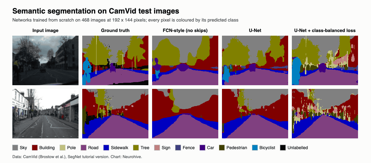
| Method | Pixel accuracy | Mean IoU | Training time |
|---|---|---|---|
| Random forest on colour + position | 67.7% | 0.251 | 1 min |
| FCN-style network, no skip connections | 83.4% | 0.396 | 11 min |
| U-Net | 86.8% | 0.483 | 12 min |
| U-Net + class-balanced loss | 80.1% | 0.476 | 12 min |
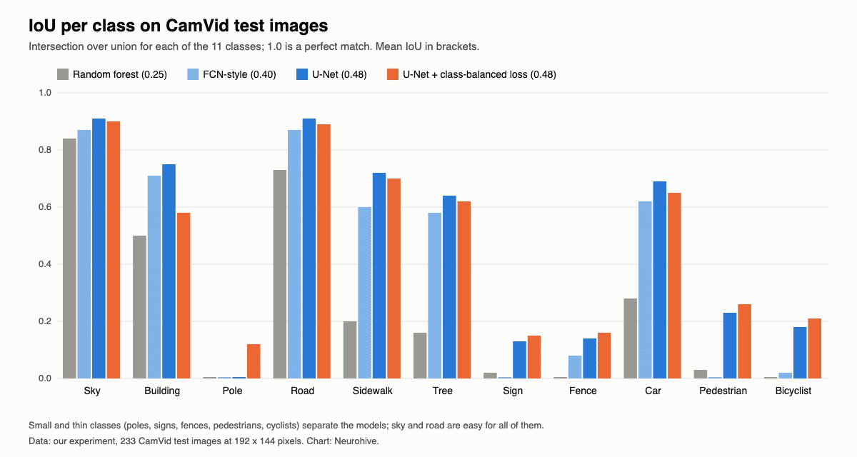
What the experiment shows:
- Context is everything. The random forest, which sees each pixel in isolation, labels two thirds of the pixels correctly, mostly sky and road, but reaches only 0.25 mean IoU. From colour alone it cannot tell a grey sidewalk from a grey road (sidewalk IoU 0.20) and finds no poles, fences or cyclists at all.
- Skip connections sharpen the result. The FCN-style network knows roughly where things are but draws blurry blobs: thin poles disappear and pedestrians merge with the background. Adding skip connections, which is all that separates it from the U-Net, raised mean IoU from 0.40 to 0.48, while pixel accuracy rose only 3.4 points. The gains came from small and thin classes: sidewalk from 0.60 to 0.72, signs from 0.00 to 0.13, pedestrians from 0.00 to 0.23 and bicyclists from 0.02 to 0.18.
- Pixel accuracy hides failures. The U-Net labels 86.8% of pixels correctly, yet its IoU for poles is 0.00 and for signs 0.13. Without per-class metrics you would not notice.
- A class-balanced loss is a trade-off, not a free gain. Weighting rare classes up made the U-Net find poles (IoU 0.00 to 0.12), more of the pedestrians and cyclists (0.23 to 0.26 and 0.18 to 0.21), but it also started to paint poles, signs and fences onto building walls: building IoU fell from 0.75 to 0.58 and pixel accuracy from 86.8% to 80.1%, with mean IoU about the same. Which model is better depends on the cost of errors: for a car, missing a cyclist is worse than mislabelling a wall.
- This is a lower bound. Our networks were small, trained from scratch on 468 images at a quarter of the original resolution for 30 epochs. Models in research papers start from encoders pretrained on large data sets and work at full resolution, and they reach well above 0.6 mean IoU on CamVid. Pretraining matters most for exactly the rare classes that our models struggle with.
Applications
- Autonomous driving and robotics. Cars and robots segment camera images into road, lane markings, sidewalk, vehicles and people to decide where they can move. Real-time models run at dozens of frames per second on in-car hardware, often together with lidar segmentation.
- Medical imaging. Segmenting organs, tumours and lesions in CT, MRI and microscopy images lets doctors measure volumes, plan radiotherapy and track disease over time. U-Net and its 3D variants, such as the self-configuring nnU-Net, are the workhorses here.
- Satellite and aerial imagery. Land-cover mapping, building footprints, crop monitoring, deforestation and flood mapping all start with per-pixel classification.
- Photo and video editing. Background removal and blur in video calls, portrait mode on phones, sky replacement and object selection in photo editors rely on segmentation, increasingly on SAM-style promptable models.
- Industry and agriculture. Inspecting surfaces for defects, measuring fruit and weeds in fields, sorting waste.
- Image restoration and generation. Segmentation masks guide inpainting and controllable image generation, and the same encoder-decoder ideas power image super resolution.
How to build a segmentation model in practice
- Try a foundation model first. If your classes can be described in words, test SAM 3 or another open-vocabulary segmenter on your images. It may solve the task without training, or produce draft masks that annotators only correct.
- Label data with masks. Annotation tools such as CVAT and Label Studio support polygons and SAM-assisted labelling. A few hundred well-labelled images are a reasonable start for a specialised task.
- Start from a pretrained model, not from scratch. Fine-tune SegFormer, Mask2Former or a DINOv3-based model with Hugging Face Transformers, or a U-Net with a pretrained encoder from the
segmentation_models_pytorchlibrary. Pretrained encoders need far less data than our from-scratch networks. - Handle imbalance and measure correctly. Use class weights or Dice loss when small classes matter, and report mean IoU and per-class IoU on a held-out test set, not only pixel accuracy.
- Optimise for deployment. For real-time use, choose a light encoder, lower the input resolution and export the model to ONNX or TensorRT; for medical images, consider nnU-Net, which configures itself for a new data set.
The basics of training such a network in PyTorch are covered in our PyTorch tutorial.
FAQ
What is the difference between semantic and instance segmentation?
Semantic segmentation gives every pixel a class but does not separate objects of the same class: two adjacent people form one “person” region. Instance segmentation outlines each object separately, person 1 and person 2, but usually ignores background “stuff” such as road or sky. Panoptic segmentation combines both.
Is semantic segmentation supervised or unsupervised?
Usually supervised: the model learns from images with pixel-level masks drawn by people. Because such labels are expensive, self-supervised pretraining, as in DINOv3, weakly supervised methods that learn from image-level tags or boxes, and automatic labelling with foundation models such as SAM are widely used to reduce the labelling effort.
What is the best model for semantic segmentation?
It depends on data and constraints. Transformer-based models such as Mask2Former and models built on large pretrained backbones lead benchmarks such as ADE20K and Cityscapes. For medical images, U-Net variants such as nnU-Net remain hard to beat. For real-time use on edge devices, light convolutional networks are still common. For open-ended classes, SAM 3 segments objects from text prompts without training.
Why use mean IoU instead of accuracy?
Because large classes dominate pixel accuracy. On street scenes, road, buildings and sky make up most pixels, so a model can score high accuracy while missing poles, signs and pedestrians entirely. Mean IoU gives every class equal weight and penalises both false positives and false negatives.
Is U-Net still used in 2026?
Yes. U-Net is the standard architecture in medical image segmentation, and many diffusion models still use it, although the newest image generators have moved to diffusion transformers. For natural images, transformer-based segmenters and foundation models have taken the lead on benchmarks, but many of them still use U-Net-style decoders.