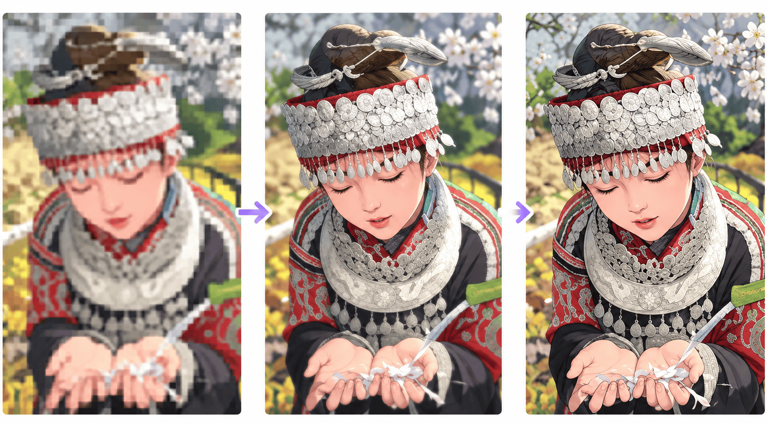
Image super resolution is the task of turning a low-resolution image into a sharper, higher-resolution one. It is what an “AI upscaler” does when it enlarges an old photo, what your phone does when you zoom past the optical limit, and what NVIDIA DLSS does in games when it renders at 1080p and shows you 4K. Unlike classic resizing, which only interpolates between the pixels you already have, a super-resolution model has learned from millions of image pairs what fine detail usually looks like, and adds it.
This guide explains how deep-learning super resolution works: how the training data is made, which network designs are used, which loss functions turn a blurry upscaler into a sharp one, and how results are measured with PSNR and SSIM. We also ran the numbers ourselves: we compared bicubic interpolation with two popular open models, SwinIR and Real-ESRGAN, on the same images, and trained a small super-resolution network in PyTorch on a laptop CPU. The code is included.
Key takeaways
- Super resolution (SR) reconstructs a high-resolution image from a low-resolution one. It is an ill-posed problem: many sharp images shrink to the same small one, so the model has to guess the missing detail from what it has learned.
- Training data is made by degrading sharp images: downscaling, blur, noise and JPEG compression.
- The loss function decides the look. Pixel losses (L1, L2) give accurate but slightly smooth results; perceptual and adversarial (GAN) losses give crisp textures that may not match the original.
- In our test at 4× scale, SwinIR beat bicubic interpolation by 2.7 dB PSNR, while Real-ESRGAN scored lower than bicubic on PSNR yet looked much sharper. This is the perception–distortion trade-off in action.
- In 2026, transformers such as HAT lead fidelity benchmarks, and one-step diffusion models lead perceptual quality for real-world photos.
What is image super resolution?
A low-resolution (LR) image can be thought of as a high-resolution (HR) image that went through some damage: it was shrunk, blurred, made noisy or compressed. In short, LR = degradation(HR). Super resolution tries to go the other way and recover HR from LR.
If we knew the exact degradation and could invert it, the problem would be easy. In practice it is ill-posed: shrinking an image by 4× in each direction throws away 15 of every 16 pixels, and countless different sharp images produce the same small one. A model therefore cannot “recover” lost detail in the strict sense. It predicts the most plausible detail based on patterns learned from training data. This is why super resolution is treated as a supervised learning problem: the model sees pairs of LR inputs and HR targets and learns the mapping between them.
The baseline that every model must beat is classical interpolation. Nearest-neighbour upscaling copies each pixel into a block and looks blocky; bilinear and bicubic interpolation compute new pixels as weighted averages of their neighbours and look smooth but blurry; Lanczos uses a wider window and is a little sharper. None of them can create a texture that is not there, which is exactly what neural networks learn to do.
Most research deals with single-image super resolution (SISR), the topic of this guide. Video super resolution can also borrow detail from neighbouring frames, and burst photography on phones merges several slightly shifted shots of the same scene.
How training data is made
Paired LR and HR photos of the same scene are hard to capture, so most training data is synthetic: you take a high-quality image and degrade it. The simplest degradation is bicubic downscaling, which is also the standard benchmark setting. More realistic pipelines add blur, sensor noise, JPEG compression artifacts and resizing with random methods.

Store the HR images losslessly (PNG rather than JPEG): otherwise the model learns to reproduce compression artifacts as if they were real detail. Common training sets are DIV2K (800 training images in 2K resolution), Flickr2K and the much larger LSDIR (about 85,000 images); results are reported on small classic test sets such as Set5, Set14, BSD100, Urban100 and Manga109.
A key insight of the past few years is that the degradation in training must match the degradation in use. A model trained only on clean bicubic downscaling works well on benchmark images but produces artifacts on real phone photos or old JPEGs, which were damaged in more complicated ways. Real-ESRGAN solved much of this in 2021 with a “high-order” degradation pipeline that applies a chain of blur, resizing, noise and JPEG compression twice, so the model sees a wide range of real-world damage during training.
From SRCNN to diffusion: a short history
Deep learning took over super resolution in 2014, and the field has gone through roughly one architecture family per era, following the rest of computer vision:
| Year | Model | What it introduced |
|---|---|---|
| 2014 | SRCNN | First deep-learning SR model: a 3-layer CNN applied to a bicubically upscaled image |
| 2016 | ESPCN, FSRCNN, VDSR | Processing at low resolution with upsampling at the end (sub-pixel convolution); deeper residual networks |
| 2017 | SRGAN, EDSR | Perceptual and adversarial losses for realistic texture; large residual networks without batch normalization |
| 2018 | RCAN, ESRGAN | Channel attention and networks with hundreds of layers; an improved GAN that won the PIRM perceptual challenge |
| 2021 | SwinIR, Real-ESRGAN, SR3 | Vision transformers for restoration; realistic degradation pipelines; early diffusion-based SR |
| 2023–2024 | HAT, StableSR, SUPIR, OSEDiff, MambaIR | Hybrid attention transformers; SR built on pretrained text-to-image diffusion models; one-step diffusion; state-space (Mamba) models |
| 2025–2026 | One-step diffusion transformers | Fast diffusion SR on large image-generation backbones such as FLUX and Qwen-Image, with control over how much detail is invented |
The state of the art is clearly visible in the NTIRE 2026 challenge on 4× super resolution, held with CVPR 2026: 194 registered participants and 31 teams with valid entries. In the fidelity track, ranked by PSNR, the winner reached 33.73 dB on the DIV2K test set with a hybrid of HAT (a transformer) and NAFNet (a CNN). In the perceptual track, the leading entries were one-step diffusion models built on large image generators, including a 4-billion-parameter FLUX.2 backbone. Transformers remain the main tool for faithful restoration; diffusion dominates when the goal is the most realistic-looking result.
Where the upsampling happens
Every SR network has to increase the image size somewhere. Where that happens is the main architectural choice, and the survey by Wang, Chen and Hoi groups networks into four frameworks.
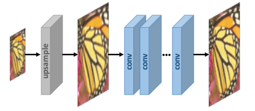
Pre-upsampling
The LR image is first enlarged with bicubic interpolation, and a CNN then refines this coarse HR image. This was SRCNN’s approach. The network only has to learn to sharpen, which is easy, and it works for any scale factor. The downside is cost: every convolution runs at full output resolution, and the network may amplify noise and blur already present in the interpolated input.
Post-upsampling
The network extracts features from the original LR image and enlarges it only in the last, learnable layer. Because almost all computation happens at low resolution, this is much faster, and it is the design used by nearly all modern models, from EDSR to SwinIR and Real-ESRGAN.
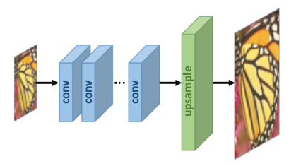
The learnable upsampling layer is usually a transposed convolution or a sub-pixel convolution (pixel shuffle). A sub-pixel layer predicts r² channels at low resolution and rearranges them into an image r times larger in each direction. It avoids the checkerboard artifacts that transposed convolutions often produce, and it is what we use in the PyTorch example below.
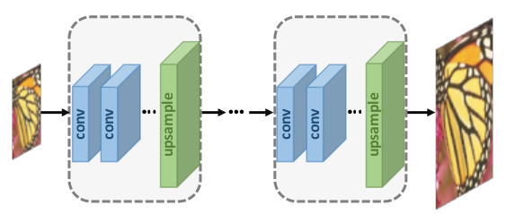
Progressive upsampling
For large factors such as 8×, a single upsampling step is hard to learn. Progressive networks such as LapSRN enlarge the image in stages, for example 2× three times, predicting extra detail at each level of a pyramid. Splitting a hard problem into easier ones makes training more stable.
Iterative up-and-down sampling
Networks such as DBPN repeatedly upsample and downsample feature maps, checking that the HR estimate is consistent with the LR input at every stage. This captures the relationship between LR and HR more precisely, at the cost of a more complex network.
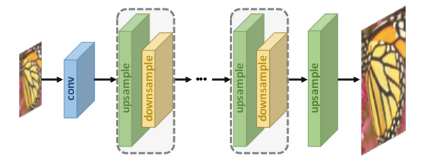
Inside these frameworks, networks use the same building blocks as the rest of deep learning: residual connections that let the network learn only the missing high-frequency detail, dense connections, attention over channels or spatial positions, and, since 2021, transformer blocks with shifted-window attention.
Loss functions
The loss function measures how far the generated image is from the real HR image, and backpropagation uses it to update the weights. In super resolution, the choice of loss has more influence on how results look than the architecture does. Models usually combine several losses with weights: total_loss = w1 * pixel_loss + w2 * perceptual_loss + w3 * adversarial_loss.
Pixel loss
The simplest option compares images pixel by pixel: L2 (mean squared error), L1 (mean absolute error) or a smooth variant. Minimizing L2 directly maximizes PSNR, the most common metric. But when the model is unsure which of many plausible textures is correct, the pixel loss is minimized by predicting their average, and an average of textures is a blur. That is why models trained only with pixel losses look accurate but slightly soft. L1 is usually preferred over L2 because it converges better and gives sharper edges.
Perceptual (content) loss
Instead of comparing pixels, compare what a pretrained image classifier “sees”. Both images are passed through a network such as VGG19, and the loss is the distance between their feature maps at layer l: ‖φl(Î) − φl(I)‖², where Î is the generated image and I the real one. Features from deeper layers capture edges, textures and shapes rather than exact pixel values, so this loss rewards images that look right to a human even if pixels are slightly shifted.
Texture (style) loss
Borrowed from neural style transfer, this loss compares Gram matrices of feature maps: Gij = Σk FikFjk, the correlations between feature channels i and j at a given layer. Matching Gram matrices makes textures statistically similar to the original, such as the same kind of fur or grass, without requiring each strand to be in the same place.
Total variation loss
Total variation (TV) is the sum of absolute differences between neighbouring pixels. Adding a small TV term suppresses noise in the output, but too much of it makes images look flat, so modern models rarely rely on it.
Adversarial loss
A generative adversarial network (GAN) adds a second network, the discriminator, which learns to tell real HR images from generated ones. The SR network, now the generator, is trained to fool it. Blurry averages are easy to spot, so the generator learns to produce sharp, realistic textures instead. SRGAN introduced this idea in 2017, and ESRGAN and Real-ESRGAN refined it.
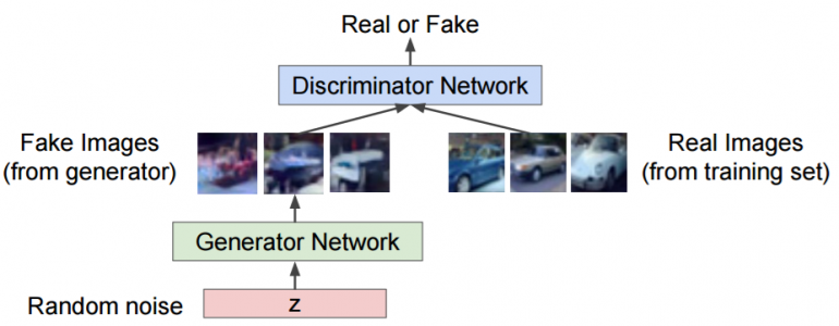
The price is fidelity: the textures look real but are partly invented, and GAN training is less stable. Diffusion models push this further. They start from a pretrained image generator that knows what photos look like and condition it on the LR input, producing even more convincing detail, including details that were never in the original scene.
How quality is measured: PSNR, SSIM and beyond
Image quality assessment (IQA) uses two kinds of metrics. Full-reference metrics compare the result with the true HR image, which is possible on benchmarks where the HR image is known. No-reference metrics estimate quality from the result alone, which is what you need for real photos without a ground truth. Human ratings, collected as a mean opinion score (MOS), remain the final judge but are slow and expensive.
PSNR
Peak signal-to-noise ratio is based on the mean squared error between the two images: PSNR = 10 · log10(MAX² / MSE), where MAX is the largest possible pixel value, 255 for 8-bit images. It is measured in decibels; higher is better, and for 4× super resolution typical values are 25–35 dB. Because it only cares about pixel differences, PSNR rewards safe, blurry predictions and correlates poorly with what people perceive. By convention, SR papers compute it on the luminance (Y) channel and ignore a border as wide as the scale factor.
SSIM
The structural similarity index compares local patterns of brightness, contrast and structure instead of raw pixel errors:
SSIM(x, y) = ((2μxμy + C1)(2σxy + C2)) / ((μx² + μy² + C1)(σx² + σy² + C2))
Here μ is the mean of a local window, σ² its variance, σxy the covariance between the two images, and C1, C2 small constants that keep the division stable. SSIM is computed over sliding windows and averaged, ranges up to 1 for identical images, and matches human judgement better than PSNR, but it still favours smooth results over invented texture.
Perceptual and no-reference metrics
Modern papers add learned metrics. LPIPS and DISTS compare deep features of the two images, much like the perceptual loss, and agree with human ratings far better than PSNR. No-reference metrics such as NIQE, MUSIQ, MANIQA and CLIP-IQA score an image’s naturalness without a reference. The NTIRE 2026 perceptual track, for example, ranked teams by a combination of LPIPS, DISTS, CLIP-IQA, MANIQA, MUSIQ and NIQE.
No single number is enough, because of the perception–distortion trade-off proved by Blau and Michaeli in 2018: beyond a certain point, an algorithm cannot improve both fidelity to the original (PSNR, SSIM) and perceived realism at the same time. That is why benchmarks now have separate fidelity and perceptual tracks, and why our test below shows two very different winners.
Our test: bicubic vs SwinIR vs Real-ESRGAN
To see the trade-off in practice, we upscaled four standard test images from scikit-image (a photo of an astronaut, a cat, a cup of coffee and a rocket launch) by 4×. Each image was first downscaled 4× with bicubic interpolation, then enlarged back with three classical methods and two open models with official weights:
- SwinIR-M (11.9 million parameters): a Swin transformer trained on DIV2K and Flickr2K with L1 pixel loss on bicubic degradation, a classic fidelity model.
- Real-ESRGAN x4plus (16.7 million parameters): a CNN trained with perceptual and GAN losses on synthetic real-world degradations, the model behind many free upscaling apps.
The script loads both models with the spandrel library, which recognizes most SR architectures from their weights, and measures PSNR and SSIM on the Y channel, as in research papers. It runs on a CPU:
import time
import numpy as np
import torch
from PIL import Image
from skimage import data
from skimage.metrics import peak_signal_noise_ratio, structural_similarity
from spandrel import ModelLoader   # pip install spandrel: loads SwinIR, ESRGAN, HAT and other SR architectures

torch.set_grad_enabled(False)
SCALE = 4

def load(path):
    state = torch.load(path, map_location="cpu", weights_only=True)
    return ModelLoader().load_from_state_dict(state).eval()

# Official weights from the GitHub releases of SwinIR and Real-ESRGAN
models = {
    "SwinIR-M (L1 loss)": load("001_classicalSR_DF2K_s64w8_SwinIR-M_x4.pth"),
    "Real-ESRGAN (GAN loss)": load("RealESRGAN_x4plus.pth"),
}
resamplers = {"Nearest neighbour": Image.NEAREST, "Bicubic": Image.BICUBIC, "Lanczos": Image.LANCZOS}

def upscale(method, lr):
    if method in resamplers:
        h, w = lr.shape[:2]
        return np.array(Image.fromarray(lr).resize((w * SCALE, h * SCALE), resamplers[method]))
    x = torch.from_numpy(lr).permute(2, 0, 1).float().unsqueeze(0) / 255.0
    y = models[method](x).clamp(0, 1)[0].permute(1, 2, 0).numpy()
    return (y * 255.0).round().astype(np.uint8)

def y_channel(img):
    """Luminance (Y of YCbCr): SR papers report PSNR and SSIM on Y."""
    img = img.astype(np.float64)
    return 16.0 + (65.481 * img[..., 0] + 128.553 * img[..., 1] + 24.966 * img[..., 2]) / 255.0

def score(sr, hr):
    a, b = y_channel(sr)[SCALE:-SCALE, SCALE:-SCALE], y_channel(hr)[SCALE:-SCALE, SCALE:-SCALE]
    return peak_signal_noise_ratio(b, a, data_range=255), structural_similarity(b, a, data_range=255)

results = {m: [] for m in [*resamplers, *models]}
seconds = {m: 0.0 for m in results}
for name in ["astronaut", "chelsea", "coffee", "rocket"]:          # test images bundled with scikit-image
    hr = getattr(data, name)()
    hr = hr[: hr.shape[0] // SCALE * SCALE, : hr.shape[1] // SCALE * SCALE]
    lr = np.array(Image.fromarray(hr).resize((hr.shape[1] // SCALE, hr.shape[0] // SCALE), Image.BICUBIC))
    for m in results:
        start = time.perf_counter()
        sr = upscale(m, lr)
        seconds[m] += time.perf_counter() - start
        results[m].append(score(sr, hr))

print(f"{'method':24s} {'PSNR, dB':>9s} {'SSIM':>7s} {'CPU s/image':>12s}")
for m, r in results.items():
    psnr, ssim = np.mean(r, axis=0)
    print(f"{m:24s} {psnr:9.2f} {ssim:7.4f} {seconds[m] / len(r):12.2f}")
method PSNR, dB SSIM CPU s/image
Nearest neighbour 27.53 0.7859 0.00
Bicubic 28.90 0.8250 0.00
Lanczos 29.10 0.8308 0.00
SwinIR-M (L1 loss) 31.59 0.8947 5.97
Real-ESRGAN (GAN loss) 27.77 0.8137 3.13SwinIR is the clear winner on the numbers: 31.59 dB, 2.7 dB above bicubic interpolation and 2.5 dB above Lanczos, with the highest SSIM. Real-ESRGAN scores 27.77 dB, lower than bicubic. By PSNR it looks like a failure. But look at the images:
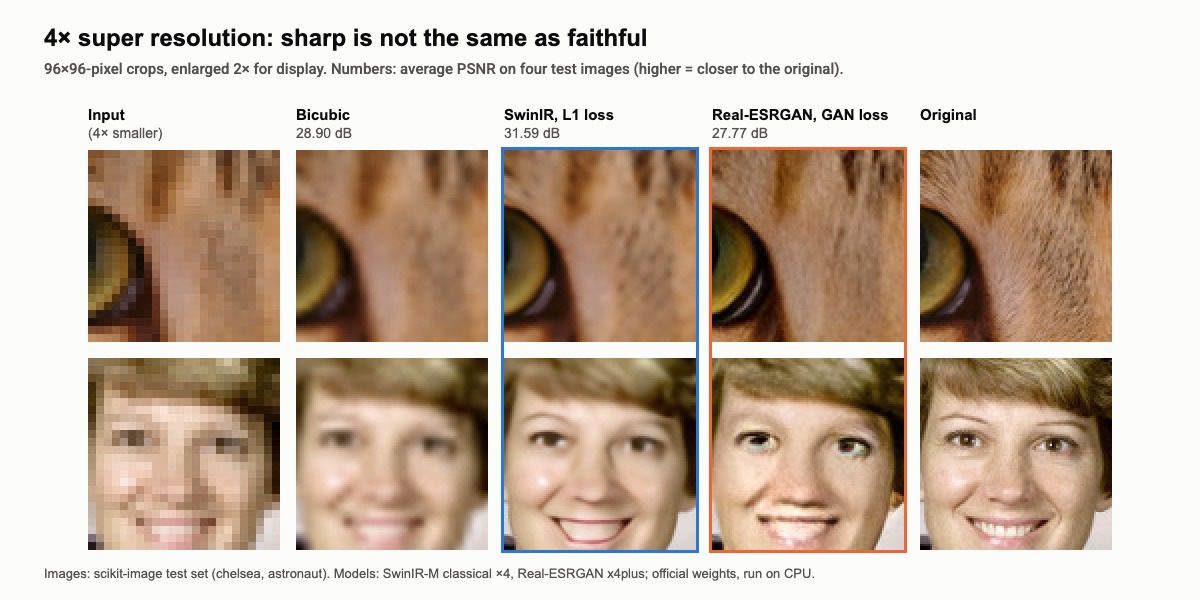
Bicubic interpolation is blurry. SwinIR restores sharp edges, the outline of the cat’s eye and the shape of the smile, but fur and skin stay smooth. Real-ESRGAN is the sharpest of all and draws convincing fur, yet it is not the original fur: strands are in different places, which costs it PSNR. On the small face, the GAN goes further and redraws the eyes and lips in a way that changes the person’s appearance. This is the core trade-off. Fidelity models are the right choice when the result must be trustworthy (medical, satellite and scientific images, document scans, evidence). Generative models are the right choice when the result must simply look good (old family photos, game textures, AI-generated art), as long as you remember that the detail is invented.
One caveat: Real-ESRGAN was trained for messy real-world degradations, not clean bicubic downscaling, so a benchmark setting like ours is not its home ground. On a real blurry, noisy JPEG it would usually beat SwinIR, which was trained only on clean data.
Train your own super-resolution model in PyTorch
To show how simple the core idea is, here is a complete ESPCN, the 2016 model that introduced sub-pixel convolution. It has three convolutional layers and 24,752 parameters, works on the luminance channel like the original paper, and trains with an L1 pixel loss on random patches from twelve other scikit-image sample images. It needs only PyTorch, scikit-image and Pillow, and trains in under three minutes on a CPU:
import time
import numpy as np
import torch
from torch import nn
from PIL import Image
from skimage import data
from skimage.metrics import peak_signal_noise_ratio

torch.manual_seed(0)
rng = np.random.default_rng(0)
SCALE = 4

def to_y(img):
    """Luminance channel in [0, 1]; ESPCN, like most classic SR models, works on Y only."""
    if img.ndim == 2:
        return img.astype(np.float32) / 255.0
    img = img[..., :3].astype(np.float32)
    return (16.0 + (65.481 * img[..., 0] + 128.553 * img[..., 1] + 24.966 * img[..., 2]) / 255.0) / 255.0

def downscale(y, scale=SCALE):
    h, w = y.shape
    return np.array(Image.fromarray(y, mode="F").resize((w // scale, h // scale), Image.BICUBIC))

# Training images: scikit-image samples that are not in the test set
train = [data.camera(), data.moon(), data.coins(), data.brick(), data.grass(), data.gravel(), data.clock(),
         data.immunohistochemistry(), data.hubble_deep_field(), data.retina()[::2, ::2], data.colorwheel(),
         data.stereo_motorcycle()[0]]
train = [to_y(im)[: im.shape[0] // SCALE * SCALE, : im.shape[1] // SCALE * SCALE] for im in train]
pairs = [(downscale(hr), hr) for hr in train]

def batch(n=64, size=24):
    """Random aligned patches: size x size from the LR image, (4*size) x (4*size) from the HR image."""
    lr_b, hr_b = [], []
    for _ in range(n):
        lr, hr = pairs[rng.integers(len(pairs))]
        y, x = rng.integers(lr.shape[0] - size), rng.integers(lr.shape[1] - size)
        lr_b.append(lr[y:y + size, x:x + size])
        hr_b.append(hr[y * SCALE:(y + size) * SCALE, x * SCALE:(x + size) * SCALE])
    return torch.tensor(np.array(lr_b)).unsqueeze(1), torch.tensor(np.array(hr_b)).unsqueeze(1)

class ESPCN(nn.Module):
    """Shi et al., 2016: features are extracted at low resolution, upsampling happens in the last layer."""
    def __init__(self, scale=SCALE):
        super().__init__()
        self.body = nn.Sequential(
            nn.Conv2d(1, 64, 5, padding=2), nn.Tanh(),
            nn.Conv2d(64, 32, 3, padding=1), nn.Tanh(),
            nn.Conv2d(32, scale * scale, 3, padding=1),
        )
        self.upsample = nn.PixelShuffle(scale)   # (16, H, W) -> (1, 4H, 4W): sub-pixel convolution

    def forward(self, x):
        return self.upsample(self.body(x))

model = ESPCN()
print("parameters:", sum(p.numel() for p in model.parameters()))
optimizer = torch.optim.Adam(model.parameters(), lr=1e-3)
scheduler = torch.optim.lr_scheduler.CosineAnnealingLR(optimizer, T_max=3000)
loss_fn = nn.L1Loss()                            # pixel loss

start = time.perf_counter()
for step in range(1, 3001):
    lr_b, hr_b = batch()
    loss = loss_fn(model(lr_b), hr_b)
    optimizer.zero_grad()
    loss.backward()
    optimizer.step()
    scheduler.step()
    if step in (1, 500, 1000, 2000, 3000):
        print(f"step {step:4d}  L1 loss {loss.item():.4f}")
print(f"training time: {time.perf_counter() - start:.0f} s on CPU")

# Test on the four images from the comparison above, PSNR on Y with a 4-pixel border removed
model.eval()
for name in ["astronaut", "chelsea", "coffee", "rocket"]:
    im = getattr(data, name)()
    hr = to_y(im)[: im.shape[0] // SCALE * SCALE, : im.shape[1] // SCALE * SCALE]
    lr = downscale(hr)
    bicubic = np.array(Image.fromarray(lr, mode="F").resize(hr.shape[::-1], Image.BICUBIC))
    with torch.no_grad():
        sr = model(torch.tensor(lr)[None, None]).clamp(0, 1)[0, 0].numpy()
    crop = lambda a: a[SCALE:-SCALE, SCALE:-SCALE]
    p_bic = peak_signal_noise_ratio(crop(hr), crop(bicubic.clip(0, 1)), data_range=1)
    p_sr = peak_signal_noise_ratio(crop(hr), crop(sr), data_range=1)
    print(f"{name:10s} bicubic {p_bic:.2f} dB   ESPCN {p_sr:.2f} dB")
parameters: 24752
step 1 L1 loss 0.4402
step 500 L1 loss 0.0384
step 1000 L1 loss 0.0273
step 2000 L1 loss 0.0248
step 3000 L1 loss 0.0232
training time: 161 s on CPU
astronaut bicubic 26.85 dB ESPCN 27.54 dB
chelsea bicubic 31.48 dB ESPCN 32.00 dB
coffee bicubic 27.29 dB ESPCN 27.70 dB
rocket bicubic 30.00 dB ESPCN 30.17 dBThe tiny network beats bicubic interpolation on all four test images, by 0.45 dB on average and by up to 0.7 dB on the astronaut photo. That is far from SwinIR’s 2.7 dB, which is expected: SwinIR has 480 times more parameters and was trained on about 3,500 high-resolution images for hundreds of thousands of iterations. Training on a real data set such as DIV2K and for longer is the main way to close the gap. If you are new to the training loop used here, see our PyTorch tutorial and PyTorch vs TensorFlow comparison, and for the hardware side, our guide to the best GPU for AI.
Real-world super resolution and diffusion models
Benchmarks with bicubic degradation are clean and reproducible, but real photos are damaged in unknown ways. Research on real-world (or blind) super resolution follows three main lines:
- Better synthetic degradations. Real-ESRGAN’s high-order pipeline and similar approaches train the model on so many kinds of damage that real images look familiar to it.
- Diffusion priors. Models such as StableSR, DiffBIR and SUPIR reuse a pretrained text-to-image diffusion model, which has seen billions of images, and condition it on the LR input. They produce remarkably natural detail, but the original versions needed dozens of denoising steps per image.
- One-step diffusion. Since OSEDiff in 2024, distillation has cut diffusion SR to a single step, making it practical. At CVPR 2026, several papers built one-step SR on large diffusion transformers. ODTSR, built on Qwen-Image, lets users adjust the balance between fidelity and invented detail, and can sharpen hard cases such as small scene text.
Unsupervised approaches, which learn from unpaired LR and HR images, and general image restoration models that handle denoising, deblurring and upscaling in one network are also active areas. An example is RealRestorer, an open model that outperformed Nano Banana Pro on a real-world restoration benchmark in March 2026.
AI upscaling tools in 2026
Most people meet super resolution through products rather than research code. A rough map of the options:
- Upscayl: a free, open-source desktop app for Windows, macOS and Linux that runs Real-ESRGAN-family models locally on your GPU.
- Topaz Gigapixel: a paid desktop app for photographers with several models, from faithful to generative.
- Magnific: a generative upscaler with a “creativity” setting that controls how much new detail is invented, popular for AI-generated art.
- Adobe Photoshop and Lightroom Super Resolution: doubles the width and height of a photo inside the Adobe workflow.
- Online services such as Krea and Let’s Enhance, and the many free web enhancers reviewed in our AI photo enhancer comparison.
- Games and video: NVIDIA DLSS renders games at a lower resolution and upscales them in real time; DLSS 4.5, announced at CES 2026, uses a second-generation transformer model. RTX Video Super Resolution upscales streaming video in browsers, and similar features exist from AMD (FSR) and Intel (XeSS).
When choosing, ask the same question as in our test: do you need the image to be faithful, or to look good? For documents, products and anything you will rely on as evidence, choose a fidelity setting. For artwork and personal photos, a generative upscaler usually gives the more pleasing result.
FAQ
What is the difference between super resolution and upscaling?
Upscaling means making an image larger by any method, including simple interpolation, which adds pixels but no detail. Super resolution is upscaling that tries to reconstruct high-frequency detail, today almost always with a neural network. “AI upscaling” is the everyday name for super resolution.
Can super resolution recover details that were not captured?
No. Information lost when an image was taken at low resolution cannot be recovered exactly. Models predict the most plausible detail based on training data. Fidelity-oriented models stay close to the evidence in the image; generative models (GANs, diffusion) invent realistic but possibly wrong detail, so do not rely on them to read a license plate or identify a face.
Which super-resolution model is best?
It depends on the goal. For the most accurate reconstruction, transformer models such as HAT and SwinIR lead benchmarks. For real-world photos, Real-ESRGAN is a fast and widely used default, and diffusion-based models such as SUPIR and newer one-step models give the most realistic detail at a higher computational cost.
What are PSNR and SSIM?
Both are full-reference metrics that compare the upscaled image with the true high-resolution image. PSNR is based on the average squared pixel error, measured in decibels; SSIM compares local brightness, contrast and structure on a scale up to 1. Higher is better for both, but both favour smooth results, so papers also report perceptual metrics such as LPIPS.
Is Real-ESRGAN still worth using in 2026?
Yes, for many tasks. It is fast, runs on modest GPUs, handles noisy and compressed photos well and powers free tools such as Upscayl. Diffusion-based upscalers produce more natural detail on difficult images, but they are slower and more likely to change the content.