Neural networks recognize faces in photos, translate text, recommend videos and power chatbots such as ChatGPT and Claude. Under the hood, every one of them runs the same simple idea: many small units, each multiplying its inputs by weights and adding them up, stacked in layers and tuned on examples until the output is right.
This guide explains what a neural network is and how it works, step by step: neurons, weights and biases, layers, forward propagation, the loss function, backpropagation and the learning rate. Along the way we compute a forward and backward pass by hand in NumPy, train a real network on handwritten digits in PyTorch, and run small experiments on learning rate, depth versus width, overfitting and the curse of dimensionality. All numbers in the article come from the code shown.
Key takeaways
- A neural network is a function with adjustable parameters. Each neuron computes a weighted sum of its inputs plus a bias and passes it through an activation function; layers of neurons turn raw input into a prediction.
- It learns by repeating three steps: a forward pass makes a prediction, a loss function measures the error, and backpropagation with gradient descent nudges every weight to reduce that error.
- The learning rate decides how big each nudge is. In our experiment, 0.1 trained well, 0.001 barely moved and 3.0 broke training completely.
- Bigger is not automatically better. A large network memorized 60 noisy training points perfectly but scored 10 points lower on new data; weight decay closed the gap.
- Different data needs different architectures: CNNs for images, RNNs and LSTMs for sequences, transformers for language, autoencoders and GANs for generation.
What is a neural network?
A neural network, or artificial neural network, is a machine learning model built from simple connected units called neurons. Each neuron takes a few numbers, combines them and passes the result on. Connected in layers, thousands or billions of such neurons can represent very complex functions: from pixel values to the word “cat”, from a sentence in English to the same sentence in French, from a prompt to the next word of an answer.
The name comes from biology. In 1943 Warren McCulloch and Walter Pitts described a mathematical model of a nerve cell, and in 1958 Frank Rosenblatt built the perceptron, the first neural network that could learn from examples. Modern networks share only the basic idea with the brain: signals flow through many simple units, and the strength of each connection is what the network learns.
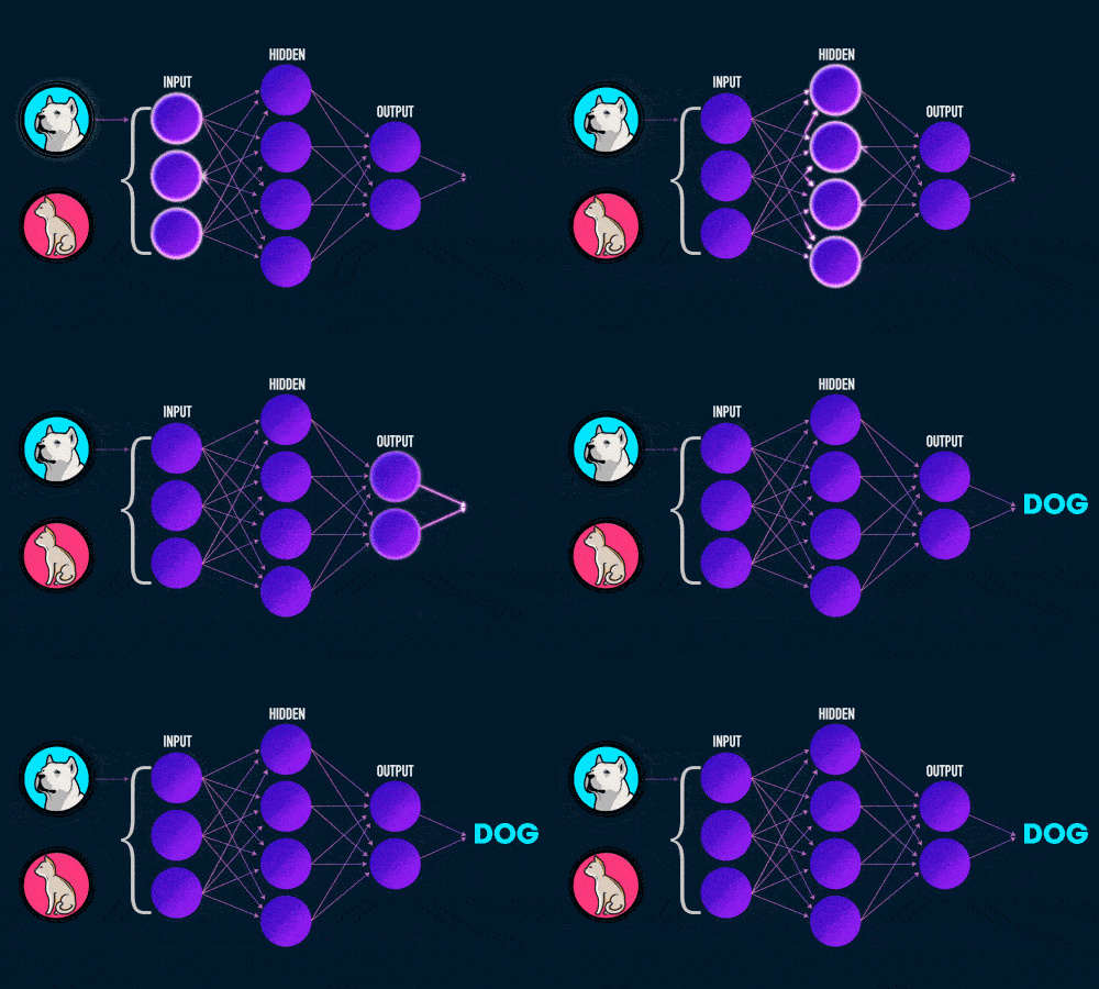
What makes neural networks useful is that nobody writes the rules by hand. You show the network examples with correct answers, for instance thousands of photos labeled “dog” or “cat”, and a training algorithm adjusts the connections until the network gives the right answers by itself. This is supervised learning, the most common way to train neural networks.
Inside a neuron: weights, bias and activation
An artificial neuron does three things:
- Multiplies each input xi by a weight wi. A weight shows how important that input is and whether it pushes the output up or down.
- Adds up the products and a bias b: z = w1x1 + w2x2 + … + wnxn + b.
- Passes the sum through an activation function: a = f(z). The result is the neuron’s output, which becomes an input for the next layer.
Weights and biases are the network’s parameters. They start as small random numbers and are what training changes. A network with 2,410 parameters, like the one we train below, has 2,410 such numbers to tune; a large language model has billions.
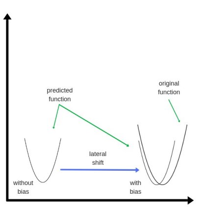
Why the bias matters. Without a bias, a neuron’s weighted sum is always zero when all inputs are zero, so the function it represents is pinned to the origin. The bias shifts the function left or right, the same way the intercept b shifts the line y = kx + b in linear regression. It lets the network fit data that does not pass through zero:
Why the activation function matters. Without it, the network would be a chain of multiplications and additions, and any number of such layers collapses into a single linear function. A nonlinear activation lets the network bend its decision boundaries and approximate curved relationships. The most popular choice in hidden layers is ReLU, f(z) = max(0, z); transformers usually use its smooth variants GELU or SiLU; output layers use sigmoid for yes/no answers and softmax for choosing among several classes.
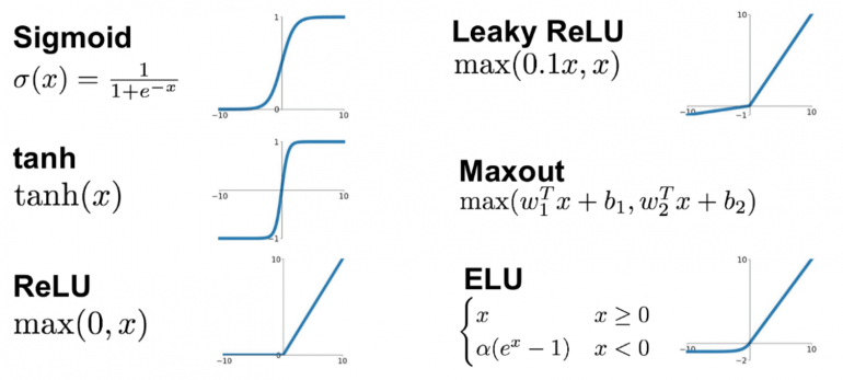
We compare these functions, with plots and code, in our guide to activation functions in neural networks.
Layers of a neural network
Neurons are organized in layers, and every neural network has three kinds of them:
- Input layer. Receives the raw data, one neuron per feature: 64 neurons for the pixels of an 8×8 image, 3 neurons for the height, weight and age of a patient. It does not compute anything, it just passes values on.
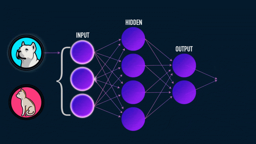
- Hidden layers. Everything between input and output. Each hidden neuron is connected to the neurons of the previous layer and learns some intermediate feature: an edge or a stroke in an image, a useful combination of numbers in a table. A network with many hidden layers is called a deep neural network, which is where the term deep learning comes from.
- Output layer. Produces the answer: one neuron with a sigmoid for “spam or not”, ten neurons with softmax for the digits 0–9, one neuron without activation for a price.
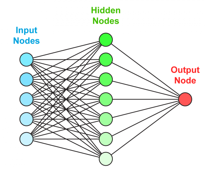
In a fully connected layer every neuron is connected to every neuron of the previous layer, so the number of parameters is easy to count: (inputs × neurons) weights plus one bias per neuron. A network with 64 inputs, 32 hidden neurons and 10 outputs has 64 × 32 + 32 = 2,080 parameters in the hidden layer and 32 × 10 + 10 = 330 in the output layer, 2,410 in total.
Forward propagation
Forward propagation, or the forward pass, is how a network turns an input into a prediction. The values flow from the input layer through the hidden layers to the output: each layer computes the weighted sums of its inputs, adds biases, applies the activation and hands the result to the next layer.
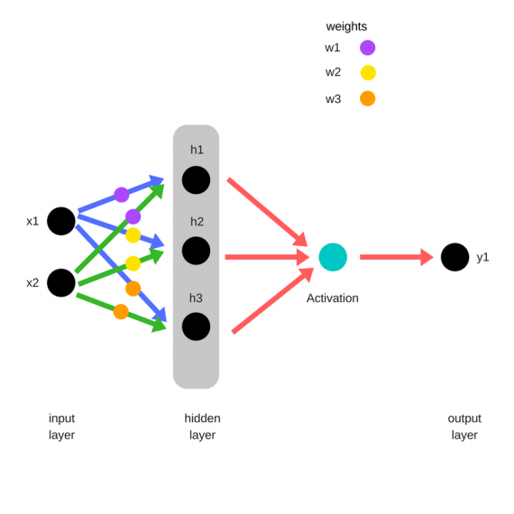
Let’s follow a tiny network with 2 inputs, 3 hidden neurons with ReLU and 1 output neuron with sigmoid. The input is x = (0.5, 0.8), the correct answer is 1. For the first hidden neuron with weights (0.2, −0.4) and bias 0.1, the weighted sum is 0.2 × 0.5 − 0.4 × 0.8 + 0.1 = −0.12. ReLU turns the negative value into 0, so this neuron stays silent. The other two hidden neurons give 0.43 and 0.15. The output neuron combines these three values with its own weights and bias, gets 0.099, and the sigmoid turns it into 0.525: the network thinks the answer is 1 with probability 52.5%. The correct answer is 1, so the prediction is weak, and training should push it up.
In matrix form, a whole layer is one line of code, h = f(W·x + b), which is why neural networks are a perfect fit for GPUs: almost all the work is matrix multiplication. If you plan to train larger models, see our guide to the best GPU for AI.
How neural networks learn
Training a neural network repeats three steps over and over, for thousands or millions of examples:
- Forward pass: compute the prediction for a batch of examples.
- Loss: compare the predictions with the correct answers using a loss function. A single number shows how wrong the network is.
- Backward pass and update: backpropagation computes, for every weight, how the loss would change if that weight changed slightly. This is the partial derivative of the loss with respect to the weight, also called the gradient. Then gradient descent moves each weight a small step in the direction that reduces the loss: w = w − η · ∂Loss/∂w, where η is the learning rate.
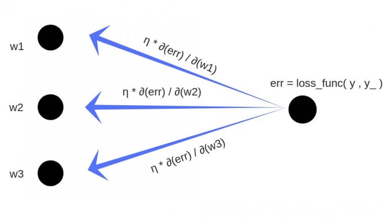
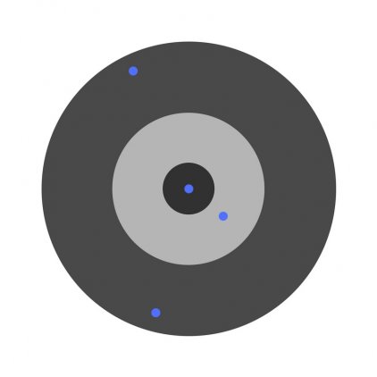
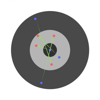
A useful analogy is a game of darts played blindfolded. Each player throws, a coach says how far and in which direction each dart missed, and every player corrects the next throw accordingly. The partial derivatives play the role of the coach: they tell each weight separately in which direction to move and how strongly it influenced the error. Weights that contributed a lot to the mistake get bigger corrections.
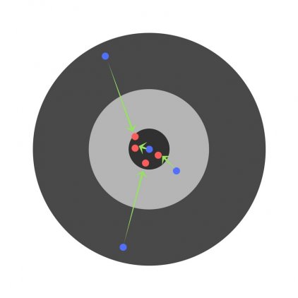
Backpropagation computes all these derivatives efficiently with the chain rule, going from the output layer back to the input, which is where the name comes from. One full pass over the training data is called an epoch; how epochs, batches and iterations relate is explained in epoch vs batch size vs iteration.
A forward and backward pass in Python
Here is the tiny network from the previous section with one complete training step: forward pass, loss, gradients by the chain rule, a numerical check of one gradient and a gradient descent update. It needs only NumPy:
import numpy as np

# A tiny network: 2 inputs -> 3 hidden neurons (ReLU) -> 1 output (sigmoid)
x = np.array([0.5, 0.8])              # one example with two features
y = 1.0                               # its correct label

W1 = np.array([[ 0.2, -0.4],          # weights of hidden neuron h1
               [ 0.7,  0.1],          # h2
               [-0.3,  0.5]])         # h3
b1 = np.array([0.1, 0.0, -0.1])       # hidden biases
W2 = np.array([0.6, -0.2, 0.9])       # output weights
b2 = 0.05                             # output bias

def relu(z):
    return np.maximum(z, 0)

def sigmoid(z):
    return 1 / (1 + np.exp(-z))

def forward(W1, b1, W2, b2):
    z1 = W1 @ x + b1                  # weighted sums of the hidden layer
    h = relu(z1)                      # hidden activations
    z2 = W2 @ h + b2                  # weighted sum of the output neuron
    p = sigmoid(z2)                   # predicted probability that y = 1
    loss = -(y * np.log(p) + (1 - y) * np.log(1 - p))   # binary cross-entropy
    return z1, h, z2, p, loss

z1, h, z2, p, loss = forward(W1, b1, W2, b2)
print("hidden pre-activations z1:", z1.round(3))
print("hidden activations h:     ", h.round(3))
print(f"output p = {p:.3f}, loss = {loss:.3f}")

# Backward pass: the chain rule, from the loss back to every weight
dz2 = p - y                           # dLoss/dz2 for sigmoid + cross-entropy
dW2 = dz2 * h
db2 = dz2
dh = dz2 * W2
dz1 = dh * (z1 > 0)                   # ReLU passes gradient only where z1 > 0
dW1 = np.outer(dz1, x)
db1 = dz1
print("dLoss/dW2:", (dW2 + 0.0).round(4))
print("dLoss/dW1:")
print((dW1 + 0.0).round(4))

# Check one gradient numerically: nudge a weight and see how the loss changes
eps = 1e-6
W1_plus = W1.copy()
W1_plus[1, 0] += eps
numeric = (forward(W1_plus, b1, W2, b2)[4] - loss) / eps
print(f"analytic dLoss/dW1[1,0] = {dW1[1, 0]:.5f}, numeric = {numeric:.5f}")

# One step of gradient descent with learning rate 0.5
lr = 0.5
W1, b1 = W1 - lr * dW1, b1 - lr * db1
W2, b2 = W2 - lr * dW2, b2 - lr * db2
print(f"loss after one update: {forward(W1, b1, W2, b2)[4]:.3f}")
hidden pre-activations z1: [-0.12 0.43 0.15]
hidden activations h: [0. 0.43 0.15]
output p = 0.525, loss = 0.645
dLoss/dW2: [ 0. -0.2044 -0.0713]
dLoss/dW1:
[[ 0. 0. ]
[ 0.0475 0.076 ]
[-0.2139 -0.3422]]
analytic dLoss/dW1[1,0] = 0.04753, numeric = 0.04753
loss after one update: 0.380Several things are worth noticing. The first hidden neuron is switched off by ReLU (its sum is −0.12), so all its gradients are exactly zero: it did not take part in this prediction and gets no blame. The analytic gradient matches the numerical estimate to five decimal places, which is the standard way to test a backpropagation implementation. And after a single update the loss drops from 0.645 to 0.380: the network now gives the correct class a higher probability. Training is nothing more than repeating this step on many examples.
Loss functions
A loss function turns the difference between predictions and correct answers into one number that training minimizes. The choice depends on the task:
| Loss function | Formula, in words | Used for |
|---|---|---|
| Mean squared error (MSE) | Average of squared differences between prediction and target | Regression: prices, temperatures, coordinates |
| Mean absolute error (MAE) | Average of absolute differences | Regression with outliers |
| Binary cross-entropy | −[y·log(p) + (1 − y)·log(1 − p)] | Yes/no classification with a sigmoid output |
| Categorical cross-entropy | −log of the probability given to the correct class | Classification into several classes with softmax; next-token prediction in language models |
| KL divergence | How much one probability distribution differs from another | Variational autoencoders, knowledge distillation |
MSE squares each error, so one large mistake costs more than several small ones:
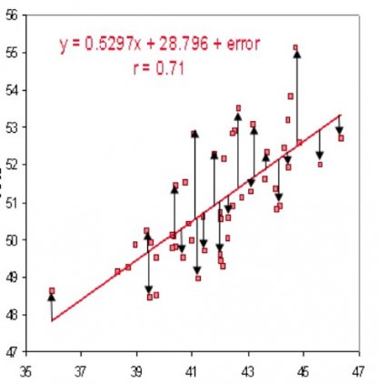
Cross-entropy punishes confident wrong answers very hard: if the network gives the correct class probability 0.01, the loss is −log(0.01) ≈ 4.6, while probability 0.9 costs only 0.1. A network that guesses randomly among 10 classes gives each class probability 0.1 and has a loss of ln 10 ≈ 2.30, a handy reference point when you watch training. KL divergence is a central part of the variational autoencoder loss.
Neural network example: recognizing handwritten digits
Now a real task. The digits dataset from scikit-learn contains 1,797 handwritten digits, each an 8×8 grayscale image. We train a network with 64 inputs, one hidden layer of 32 ReLU neurons and 10 outputs in PyTorch. The training loop is exactly the three steps from above:
import torch
from torch import nn
from sklearn.datasets import load_digits
from sklearn.model_selection import train_test_split

torch.manual_seed(0)
X, y = load_digits(return_X_y=True)            # 1,797 handwritten digits, 8x8 pixels each
X = torch.tensor(X / 16.0, dtype=torch.float32)  # scale pixel values to 0..1
y = torch.tensor(y)
X_train, X_test, y_train, y_test = train_test_split(X, y, test_size=0.25, random_state=0)

model = nn.Sequential(
    nn.Linear(64, 32),   # input layer: 64 pixels -> 32 hidden neurons
    nn.ReLU(),
    nn.Linear(32, 10),   # output layer: one score per digit 0-9
)
loss_fn = nn.CrossEntropyLoss()
optimizer = torch.optim.SGD(model.parameters(), lr=0.1)
print("parameters:", sum(p.numel() for p in model.parameters()))

for epoch in range(1, 41):
    order = torch.randperm(len(X_train))         # shuffle the training set every epoch
    total = 0.0
    for i in range(0, len(X_train), 32):         # mini-batches of 32 examples
        idx = order[i:i + 32]
        loss = loss_fn(model(X_train[idx]), y_train[idx])   # 1. forward pass and loss
        optimizer.zero_grad()
        loss.backward()                          # 2. backpropagation computes gradients
        optimizer.step()                         # 3. gradient descent updates the weights
        total += loss.item() * len(idx)
    if epoch in (1, 5, 10, 20, 40):
        with torch.no_grad():
            acc = (model(X_test).argmax(1) == y_test).float().mean()
        print(f"epoch {epoch:2d}  train loss {total / len(X_train):.3f}  test accuracy {acc:.3f}")
parameters: 2410
epoch 1 train loss 2.227 test accuracy 0.173
epoch 5 train loss 0.569 test accuracy 0.898
epoch 10 train loss 0.243 test accuracy 0.936
epoch 20 train loss 0.129 test accuracy 0.956
epoch 40 train loss 0.068 test accuracy 0.964At the start the network guesses randomly: the loss is close to ln 10 and test accuracy after one epoch is 17%. After 10 epochs it recognizes 94% of digits it has never seen, after 40 epochs 96%. Test accuracy fluctuates by a point or two from epoch to epoch because each mini-batch gives a slightly different, noisy gradient. A convolutional neural network would do better on images, but even this small fully connected network learns the task in a few seconds on a CPU.
Learning rate
The learning rate sets the size of each gradient descent step and is usually the first hyperparameter to tune. If it is too small, training crawls. If it is too large, each step overshoots the minimum: the loss jumps up and down or the weights fly off to values from which the network cannot recover.
We trained the digits network from the previous section with five learning rates, three random seeds each, for 30 epochs:
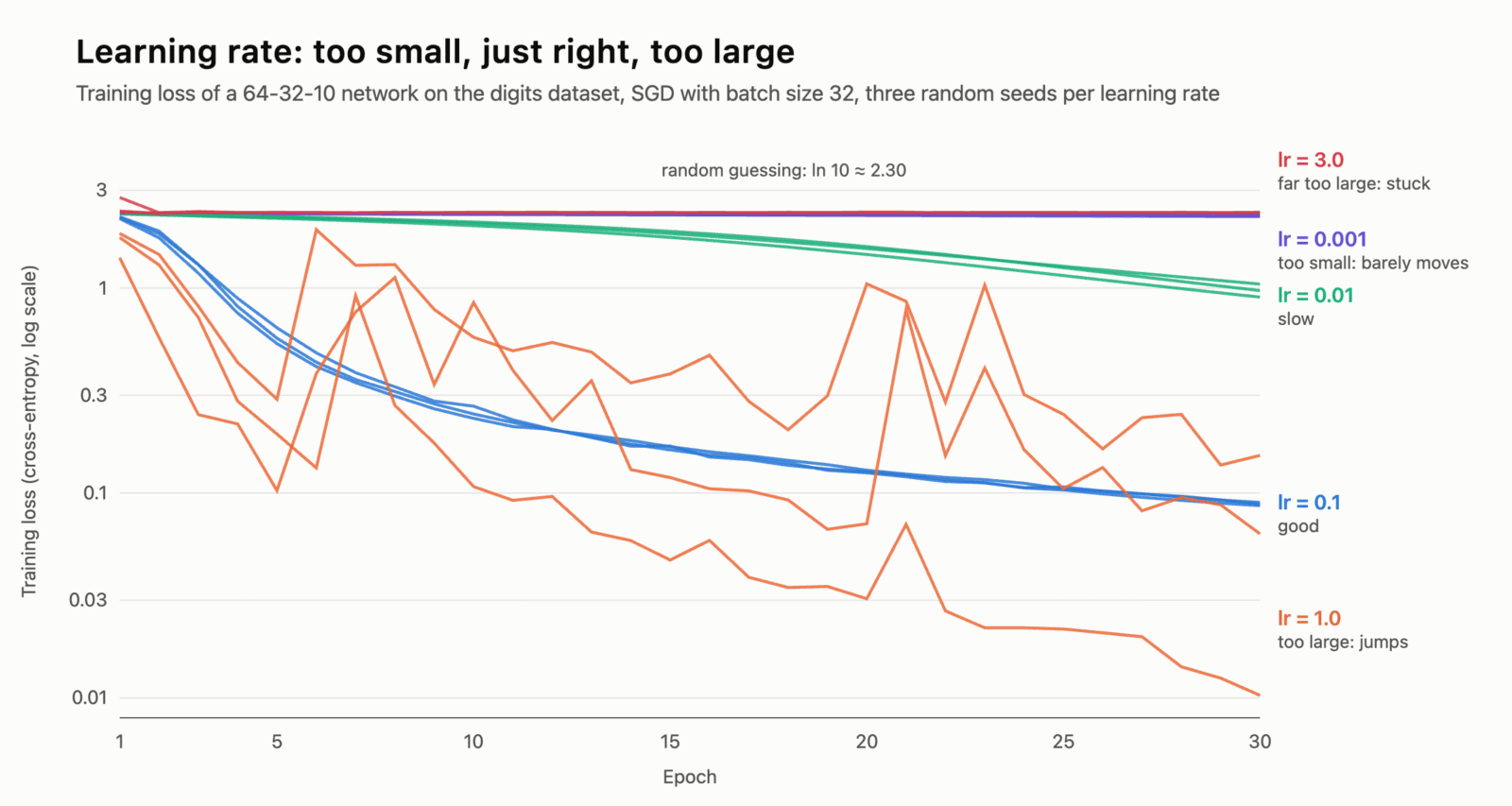
- 0.001: after 30 epochs the loss has barely moved from 2.3 and test accuracy is 14–18%, close to random guessing.
- 0.01: learning is steady but slow: loss about 1.0 and accuracy 81–87%. It needs many more epochs.
- 0.1: fast and smooth, all three runs reach a loss of about 0.09 and 91–97% test accuracy.
- 1.0: the loss repeatedly jumps up. Two runs ended at 96% accuracy, but the third ended at 21% because its last steps landed in a bad spot.
- 3.0: training breaks in the first epoch. The loss stays at the random-guessing level of about 2.33 and accuracy is 8–12%.
There is no universal best value: it depends on the model, the optimizer, the batch size and the data. A common practice is to try values on a logarithmic scale (0.001, 0.003, 0.01, 0.03…) and pick the largest one that trains stably. Adaptive optimizers such as Adam usually start around 0.001, and learning rate schedules lower the rate during training, with a short warmup at the beginning for large models. More on this in our article on gradient descent.
Types of neural networks
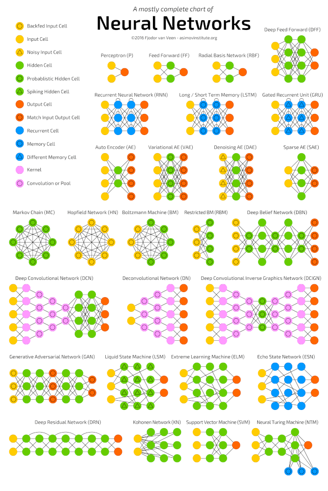
The simple fully connected network above is called a multilayer perceptron (MLP) or feedforward network. Other architectures change how neurons are connected to suit a particular kind of data:
- Multilayer perceptron (MLP): fully connected layers; works for tables and as a building block inside larger models. See the perceptron.
- Convolutional neural network (CNN): small filters slide over an image and detect local patterns; the standard tool for images and video. See how CNNs work.
- Recurrent neural network (RNN): processes sequences step by step and keeps a hidden state as memory. See the recurrent neural network.
- LSTM and GRU: recurrent networks with gates that let them remember information over long sequences. See LSTM.
- Transformer: uses attention to let every element of a sequence look at every other one; the architecture behind large language models and most modern AI.
- Autoencoders and VAE: compress the input into a small code and reconstruct it; used for compression, denoising and generation. See the variational autoencoder.
- Generative adversarial network (GAN): a generator and a discriminator compete, and the generator learns to create realistic images. See GANs.
- Graph neural networks and diffusion models: networks for data shaped as graphs, such as molecules, and the models behind modern image and video generators.
The Asimov Institute’s well-known “Neural Network Zoo” chart shows dozens of architectures as diagrams of cells and connections:
Deep vs wide neural networks
There are two ways to make a network bigger: add more neurons to a layer, making it wider, or add more layers, making it deeper.
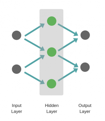
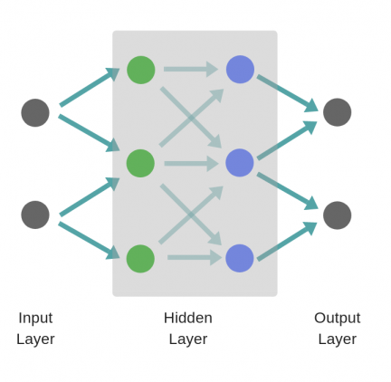
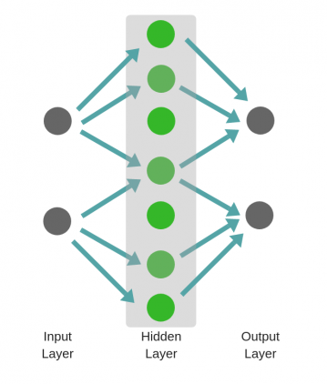
In theory, width alone is enough. The universal approximation theorem (Cybenko, 1989; Hornik, 1991) says that a network with a single hidden layer can approximate any continuous function as closely as you like, if it has enough neurons. In practice, “enough” can mean an enormous number, while a deeper network can represent the same function with far fewer parameters, because each layer builds on the features of the previous one: edges become shapes, shapes become objects.
Depth has a price: deep narrow networks are harder to train. We checked this on two interleaved spirals, a classic task that no straight line can solve. A wide network with one hidden layer of 40 neurons and a deep network with three hidden layers of 8 neurons have almost the same number of parameters; each was trained five times with different random seeds:
wide: 1 hidden layer x 40   161 parameters  test accuracy over 5 seeds: median 0.897, best 0.991, worst 0.726
deep: 3 hidden layers x 8   177 parameters  test accuracy over 5 seeds: median 0.790, best 1.000, worst 0.729
The deep network reached the best result, a perfect 100%, which the wide one never did. But it was also less reliable: in three runs out of five it got stuck below 80%. This is the trade-off in a nutshell: depth gives more expressive power per parameter, width makes optimization easier. Modern architectures get both by making networks deep and fairly wide and adding tools that keep training stable: residual connections, normalization layers and careful initialization. That is how transformers with dozens of layers and CNNs with more than a hundred are trained reliably.
Bias-variance tradeoff: underfitting and overfitting
The goal of training is not to do well on the training data but to do well on new data. Two things can go wrong:
- Underfitting (high bias): the model is too simple for the data. It makes systematic errors, and both training and test scores are low.
- Overfitting (high variance): the model is so flexible that it memorizes the training examples, including their noise. The training score is excellent, the test score is noticeably worse, and the result changes a lot with a different sample of training data.
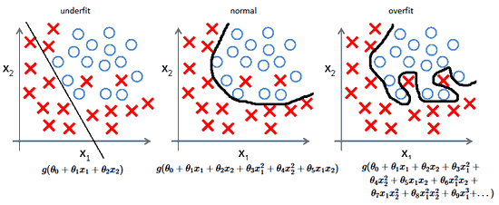
The bias-variance tradeoff describes the balance between the two: making a model more flexible reduces bias but increases variance. We reproduced the classic picture with a neural network. The training set has only 60 noisy points from the two moons dataset; accuracy is measured on 2,000 new points:
import torch
from torch import nn
from sklearn.datasets import make_moons

torch.manual_seed(0)
X_train, y_train = make_moons(n_samples=60, noise=0.25, random_state=1)   # only 60 noisy training points
X_test, y_test = make_moons(n_samples=2000, noise=0.25, random_state=2)
X_train, X_test = (torch.tensor(a, dtype=torch.float32) for a in (X_train, X_test))
y_train, y_test = (torch.tensor(a, dtype=torch.float32) for a in (y_train, y_test))

def fit(model, weight_decay=0.0, steps=1500):
    opt = torch.optim.AdamW(model.parameters(), lr=0.01, weight_decay=weight_decay)
    loss_fn = nn.BCEWithLogitsLoss()
    for _ in range(steps):
        loss = loss_fn(model(X_train).squeeze(1), y_train)
        opt.zero_grad(); loss.backward(); opt.step()
    with torch.no_grad():
        acc = lambda X, y: ((model(X).squeeze(1) > 0).float() == y).float().mean().item()
        return acc(X_train, y_train), acc(X_test, y_test)

big = lambda: nn.Sequential(nn.Linear(2, 256), nn.ReLU(), nn.Linear(256, 256), nn.ReLU(), nn.Linear(256, 1))
models = {
    "no hidden layer (too simple)":     (nn.Linear(2, 1), 0.0),
    "2 x 256 neurons, no regularization": (big(), 0.0),
    "2 x 256 neurons, weight decay":      (big(), 3.0),
}
for name, (model, wd) in models.items():
    train_acc, test_acc = fit(model, wd)
    print(f"{name:36s} train {train_acc:.3f}  test {test_acc:.3f}  gap {train_acc - test_acc:+.3f}")
no hidden layer (too simple) train 0.850 test 0.854 gap -0.004
2 x 256 neurons, no regularization train 1.000 test 0.896 gap +0.104
2 x 256 neurons, weight decay train 0.933 test 0.932 gap +0.001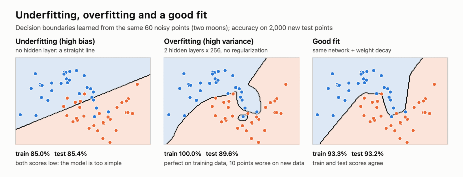
A network without hidden layers can only draw a straight line, so it underfits: 85% on both sets. A network with two hidden layers of 256 neurons, about 67,000 parameters for 60 points, bends its boundary around every noisy point and gets 100% on training data, but only 89.6% on new data. The same network with weight decay, which penalizes large weights and pushes the network toward simpler functions, draws a smooth boundary and reaches 93.2% on test data.
So the cure for overfitting is not necessarily a smaller network. In modern deep learning it is common to use a large network and control it with regularization:
- more training data or data augmentation;
- weight decay (L2 regularization) and dropout;
- early stopping: stop training when the validation loss stops improving, as shown in epoch vs batch size vs iteration;
- a validation set that is never used for training, to see overfitting when it starts.
Underfitting has the opposite cures: a bigger or deeper model, better features, longer training or less regularization.
The curse of dimensionality
Every input feature adds a dimension to the space the network has to learn in, and with each dimension the space grows exponentially. To cover a line segment with points spaced 0.1 apart you need 10 points; to cover a square, 100; a 10-dimensional cube, 10 billion. Data becomes sparse, and distances stop being informative: in high dimensions almost all points are roughly the same distance from each other. A quick check with random points:
import numpy as np

rng = np.random.default_rng(0)
for d in (2, 10, 100, 1000):
    points = rng.random((1000, d))                 # 1,000 random points in a d-dimensional cube
    query = rng.random(d)
    dist = np.linalg.norm(points - query, axis=1)
    print(f"{d:5d} dimensions: nearest / farthest distance = {dist.min() / dist.max():.2f}")
2 dimensions: nearest / farthest distance = 0.01
10 dimensions: nearest / farthest distance = 0.22
100 dimensions: nearest / farthest distance = 0.72
1000 dimensions: nearest / farthest distance = 0.90In two dimensions the nearest point is a hundred times closer than the farthest one; in 1,000 dimensions the nearest point is 90% as far as the farthest. This is the curse of dimensionality, and it is the reason why models that rely only on distances, such as k-nearest neighbors, struggle with raw high-dimensional data.
Neural networks cope better because real data is not random: a photo with a million pixels lies on a much lower-dimensional surface of “natural images”, and architectures like CNNs build in assumptions about that structure, such as locality and translation invariance. Still, more features without more data easily lead to overfitting, so feature selection, dimensionality reduction and regularization remain important.
FAQ
What is a neural network in simple terms?
A neural network is a program that learns from examples. It consists of many small units, neurons, connected in layers. Each neuron multiplies its inputs by weights, adds them up and passes the result on. During training, the weights are adjusted step by step until the network produces correct answers for the examples it has seen, and, if training went well, for new ones too.
How does a neural network learn?
By repeating three steps: it makes a prediction (forward pass), a loss function measures the error, and backpropagation calculates how each weight contributed to the error, so that gradient descent can adjust all weights slightly in the direction that reduces it. Repeated over many examples and epochs, these small adjustments add up to a model that works.
What are the three layers of a neural network?
The input layer receives the data, one or more hidden layers transform it into useful features, and the output layer produces the prediction. A network can have many hidden layers; then it is called deep.
What is the difference between a neural network and deep learning?
Deep learning is the part of machine learning that uses neural networks with many layers. Every deep learning model is a neural network, but a network with one hidden layer is usually not called deep.
How many layers and neurons does a neural network need?
There is no formula. For tabular data, one to three hidden layers with tens to hundreds of neurons are a reasonable start. For images, text and audio, people take a proven architecture, such as a CNN or a transformer, often pretrained. Start small, check whether the model underfits or overfits, and change the size accordingly.
Is a neural network the same as AI?
No. Artificial intelligence is the broad field of making machines perform tasks that need intelligence. Machine learning is a part of it, and neural networks are one family of machine learning models. They are, however, behind most of today’s AI systems, from image recognition to large language models. Simpler methods such as decision trees and gradient boosting are still often better on tabular data.