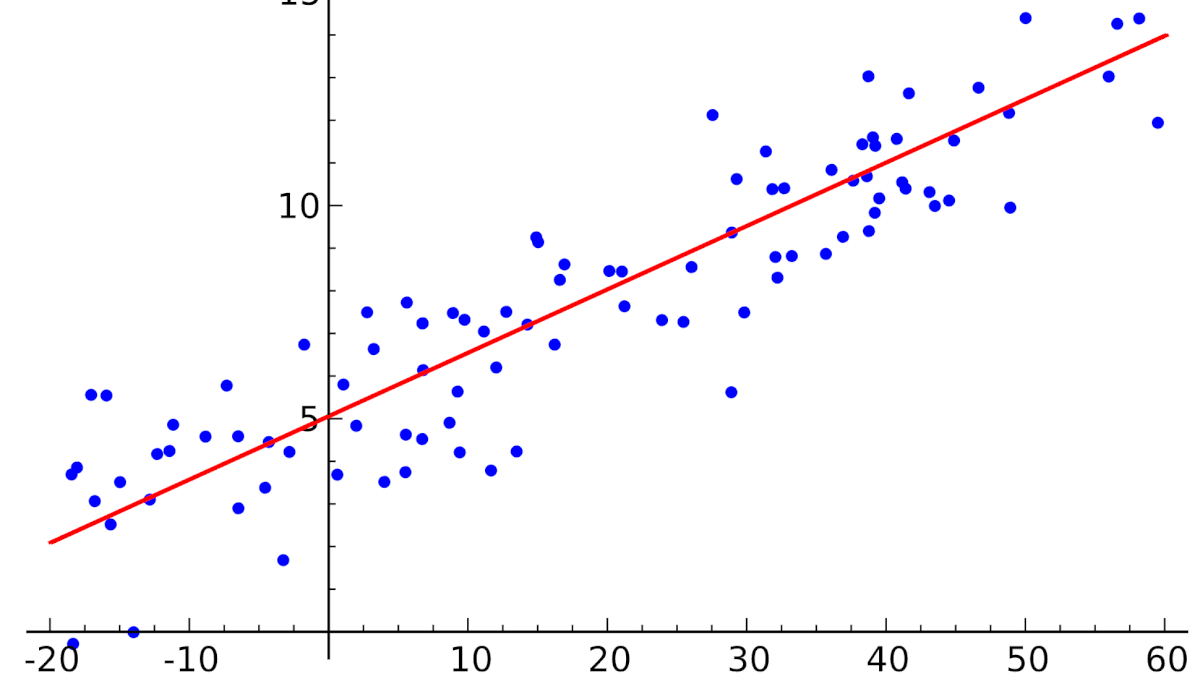
Linear regression is a machine learning model that predicts a numeric value as a weighted sum of input features plus a constant: ŷ = w₁x₁ + w₂x₂ + … + wₙxₙ + b. With one feature it fits a straight line through the data — the line of best fit; with several it fits a plane or hyperplane. The weights are chosen to minimize the mean squared error between predictions and actual values, either exactly with the least squares formula or iteratively with gradient descent. Linear regression is the simplest supervised learning algorithm, one of the most widely used models in statistics and data science, and the building block from which neural networks grow.
This guide explains linear regression step by step: the equation, a worked example with numbers, the mean squared error and why it forms a bowl, multiple linear regression, the normal equation and gradient descent, evaluation with R², the assumptions behind the model, polynomial, Ridge and Lasso regression, the difference from logistic regression, and complete Python code with NumPy and scikit-learn.
Key takeaways
- Model:
ŷ = Xw + b— each feature is multiplied by a coefficient, and the products are summed with an intercept. - Training means finding the coefficients that minimize the mean squared error, the method of least squares.
- The loss is convex: it has a single minimum, which the normal equation finds exactly and gradient descent finds iteratively.
- Evaluate with RMSE, which is in the units of the target, and R², the share of variance explained.
- Regularization (Ridge, Lasso) keeps coefficients small and helps with many or correlated features.
What Is Linear Regression?
Regression is the task of predicting a continuous number: a price, a temperature, a salary, the progression of a disease. Linear regression assumes that the target y depends on the features x linearly, so that it can be written as
ŷ = w₁x₁ + w₂x₂ + … + wₙxₙ + b
The x values are the features (also called independent variables, predictors or regressors), y is the target (dependent variable), the w values are the coefficients or weights, and b is the intercept, or bias. A coefficient says how much the prediction changes when its feature increases by one unit and all other features stay the same, which makes linear models unusually easy to interpret.
The method is old: Adrien-Marie Legendre published least squares in 1805 and Carl Friedrich Gauss in 1809, and the word “regression” comes from Francis Galton’s studies of heredity in the 1880s. It remains the first model to try on any regression problem and the baseline every more complex model has to beat.
Simple Linear Regression: A Worked Example
With a single feature, the model is the equation of a straight line, ŷ = m·x + b, where m is the slope and b the intercept. Take eight people with their years of experience and their salary in thousands of dollars. The goal is to find the line that fits these points best. Some candidate lines are clearly bad; the question is how to measure “best”:
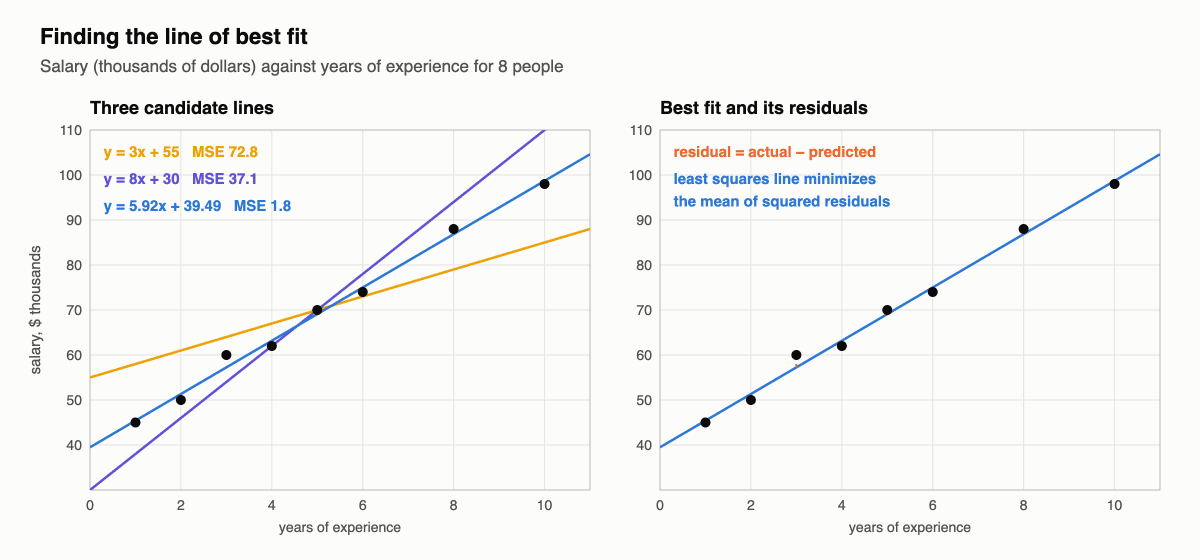
For each point, the residual is the difference between the actual value and the prediction, y − ŷ, shown by the dashed lines on the right. A good line makes the residuals small. For simple linear regression, the line that minimizes the sum of squared residuals has a closed-form solution:
m = Σ (xᵢ − x̄)(yᵢ − ȳ) / Σ (xᵢ − x̄)² b = ȳ − m · x̄
where x̄ and ȳ are the means. In Python:
import numpy as np

# Years of experience and salary (thousands of dollars) for 8 people
x = np.array([1, 2, 3, 4, 5, 6, 8, 10], dtype=float)
y = np.array([45, 50, 60, 62, 70, 74, 88, 98], dtype=float)

# Closed-form least squares for one feature
m = np.sum((x - x.mean()) * (y - y.mean())) / np.sum((x - x.mean()) ** 2)
b = y.mean() - m * x.mean()

y_pred = m * x + b
mse = np.mean((y - y_pred) ** 2)
r2 = 1 - np.sum((y - y_pred) ** 2) / np.sum((y - y.mean()) ** 2)
print(f"y = {m:.2f} * x + {b:.2f}")
print(f"MSE = {mse:.2f}, RMSE = {np.sqrt(mse):.2f}, R^2 = {r2:.3f}")
print(f"prediction for 7 years: {m * 7 + b:.1f}")
Output:
y = 5.92 * x + 39.49
MSE = 1.81, RMSE = 1.35, R^2 = 0.994
prediction for 7 years: 81.0
The model says that each additional year of experience adds about $5,920 to the salary, starting from about $39,490 for no experience, and it predicts $81,000 for someone with seven years. The three lines in the left chart have mean squared errors of 72.8, 37.1 and 1.8: the least squares line is far better than the other two.
The Loss Function: Least Squares
A loss function measures how wrong the model is on the data. Linear regression usually uses the mean squared error (MSE):
MSE = (1/n) · Σ (yᵢ − ŷᵢ)²
Squaring makes all errors positive, punishes large errors more than small ones, and gives a smooth function with a simple derivative. Minimizing the MSE is the method of ordinary least squares (OLS). When the errors are normally distributed, least squares is also the maximum likelihood solution, which is one reason it is the default. Other losses are possible: the mean absolute error is less sensitive to outliers, and the Huber loss combines the two.
Why the Error Is a Bowl
Every pair of values (m, b) defines a line and therefore an MSE. Plotting the MSE for all combinations shows its shape: an elongated bowl with a single lowest point.
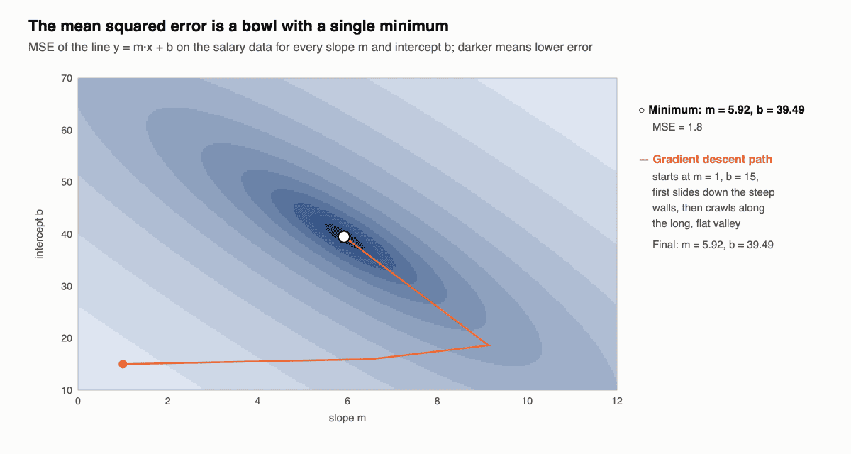
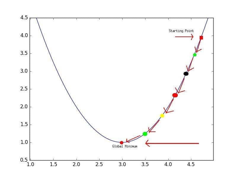
Training means finding the bottom of this bowl. The same holds with any number of features: the MSE of a linear model is always a convex function of the coefficients — a bowl in many dimensions, or a hyper-bowl. A convex function has a single global minimum, and every path downhill leads to it:
The orange path in the contour plot is gradient descent starting from m = 1, b = 15. It quickly slides down the steep walls of the bowl and then crawls along its long, flat valley, but it ends exactly at the least squares solution. The valley is elongated because the slope and the intercept are on very different scales — a reason to standardize features before using gradient descent.
Multiple Linear Regression
With n features the model becomes
ŷ = w₁x₁ + w₂x₂ + … + wₙxₙ + b
A standard trick simplifies the notation: treat the intercept b as one more weight w₀ that is always multiplied by a constant input x₀ = 1. Then the whole model is a dot product, and for a dataset stored as a matrix X with a column of ones, all predictions are computed at once:
ŷ = X · w
Adding dimensions sounds like it should make the problem much harder, but the formulation stays exactly the same in 2, 3 or 1,000 dimensions: the loss is still a convex bowl, and the goal is still its lowest point.
Normal Equation vs Gradient Descent
There are two ways to find the minimum.
The normal equation solves the problem analytically. Setting the gradient of the MSE to zero gives
w = (Xᵀ X)⁻¹ Xᵀ y
which yields the exact solution in one step. In practice libraries do not invert the matrix but use more stable methods such as QR or singular value decomposition, as numpy.linalg.lstsq and scikit-learn’s LinearRegression do.
Gradient descent starts from arbitrary coefficients and repeatedly moves them against the gradient of the loss, ∇MSE = (2/n) · Xᵀ(Xw − y), until it reaches the bottom of the bowl.
| Normal equation | Gradient descent | |
|---|---|---|
| Result | Exact solution in one step | Converges iteratively |
| Hyperparameters | None | Learning rate, number of steps |
| Feature scaling | Not needed | Strongly recommended |
| Cost | Grows with the cube of the number of features | Grows linearly; works with mini-batches and streaming data |
| Best for | Up to thousands of features | Very large datasets, online learning, models beyond linear regression |
Linear Regression in Python
The diabetes dataset in scikit-learn describes 442 patients with 10 features — age, sex, body mass index, blood pressure and six blood measurements — and a target that measures disease progression one year later. The code below fits linear regression three ways — with scikit-learn, with the normal equation and with gradient descent — and checks that all three agree:
import numpy as np
from sklearn.datasets import load_diabetes
from sklearn.linear_model import LinearRegression
from sklearn.model_selection import train_test_split
from sklearn.preprocessing import StandardScaler
from sklearn.metrics import mean_squared_error, r2_score

X, y = load_diabetes(return_X_y=True)          # 442 patients, 10 features
X_train, X_test, y_train, y_test = train_test_split(X, y, test_size=0.2, random_state=0)
scaler = StandardScaler().fit(X_train)         # same scale for every feature
X_train, X_test = scaler.transform(X_train), scaler.transform(X_test)

# 1) scikit-learn
model = LinearRegression().fit(X_train, y_train)
pred = model.predict(X_test)
print(f"test R^2 = {r2_score(y_test, pred):.3f}, RMSE = {mean_squared_error(y_test, pred) ** 0.5:.1f}")

# 2) Normal equation: add a column of ones for the intercept and solve least squares
Xb = np.c_[np.ones(len(X_train)), X_train]
w = np.linalg.lstsq(Xb, y_train, rcond=None)[0]

# 3) Gradient descent on the same mean squared error
w_gd = np.zeros(Xb.shape[1])
for step in range(5000):
    grad = 2 / len(Xb) * Xb.T @ (Xb @ w_gd - y_train)
    w_gd -= 0.1 * grad

print("sklearn vs normal equation, max difference:", round(np.abs(w[1:] - model.coef_).max(), 6))
print("normal equation vs gradient descent:       ", round(np.abs(w - w_gd).max(), 6))
top = sorted(zip(load_diabetes().feature_names, model.coef_), key=lambda t: -abs(t[1]))[:3]
print("largest coefficients:", ", ".join(f"{name} {c:.1f}" for name, c in top))
Output:
test R^2 = 0.332, RMSE = 58.5
sklearn vs normal equation, max difference: 0.0
normal equation vs gradient descent:        0.002435
largest coefficients: s5 35.8, s1 -31.2, bmi 27.5
All three methods find the same coefficients: scikit-learn and the normal equation match exactly, and gradient descent agrees to within 0.003. Because the features were standardized, the coefficients are comparable: s5, a blood serum measurement, and body mass index have the largest positive effects on the predicted progression.
Evaluating the Model: RMSE and R²
- MSE is the loss itself; it is in squared units and hard to interpret directly.
- RMSE, the square root of the MSE, is in the same units as the target: on average, predictions are off by about this much. The diabetes model has an RMSE of 58.5 on a target that ranges from 25 to 346.
- MAE, the mean absolute error, is the average size of the errors and is less affected by a few large ones.
- R², the coefficient of determination, is
1 − Σ(y − ŷ)² / Σ(y − ȳ)²: the share of the variance in the target explained by the model. An R² of 1 means perfect predictions, 0 means no better than always predicting the mean, and it can be negative on test data for a model worse than that.
The salary example has an R² of 0.994 because the data is almost perfectly linear. The diabetes model explains only 33% of the variance on unseen patients: disease progression depends on much more than ten measurements. Always compute these metrics on a test set the model did not see during training.
Assumptions of Linear Regression
Linear regression gives reliable predictions, and especially reliable confidence intervals and p-values for its coefficients, when these assumptions hold:
- Linearity: the relationship between the features and the target is linear. A curved pattern in a plot of residuals against predictions is a warning sign.
- Independence: the errors of different observations are independent — often violated in time series, where consecutive errors are correlated.
- Homoscedasticity: the errors have the same variance everywhere. A funnel shape in the residual plot means the variance grows with the prediction.
- Normality of errors: the residuals are roughly normally distributed; this matters mostly for statistical tests and intervals.
- No strong multicollinearity: the features are not highly correlated with each other. Otherwise the coefficients become unstable and hard to interpret, even if predictions stay good.
Violations do not make the model useless, but they call for remedies: transforming features or the target, adding interaction or polynomial terms, using robust errors, or switching to regularized or nonlinear models.
Polynomial, Ridge and Lasso Regression
Polynomial regression fits curves while remaining linear regression: you add new features such as x² and x³, and the model is still linear in its coefficients, so the same least squares machinery applies. In scikit-learn, combine PolynomialFeatures with LinearRegression. High degrees overfit quickly.
Regularization adds a penalty on the size of the coefficients to the loss:
- Ridge regression (L2) adds
α · Σ wᵢ². It shrinks all coefficients towards zero, stabilizes the solution when features are correlated and reduces overfitting. - Lasso regression (L1) adds
α · Σ |wᵢ|. It can set coefficients exactly to zero, so it also selects features. - Elastic Net combines both penalties.
On the standardized diabetes data, the effect is easy to see:
import numpy as np
from sklearn.datasets import load_diabetes
from sklearn.linear_model import LinearRegression, Ridge, Lasso
from sklearn.preprocessing import StandardScaler

X, y = load_diabetes(return_X_y=True)
X = StandardScaler().fit_transform(X)
for name, model in [("OLS", LinearRegression()), ("Ridge", Ridge(alpha=10)), ("Lasso", Lasso(alpha=5))]:
    coef = model.fit(X, y).coef_
    print(f"{name:>5}: sum |coef| = {np.abs(coef).sum():6.1f}, zero coefficients = {np.sum(coef == 0)}")
Output:
  OLS: sum |coef| =  164.6, zero coefficients = 0
Ridge: sum |coef| =  105.0, zero coefficients = 0
Lasso: sum |coef| =   65.0, zero coefficients = 5
Ridge makes the coefficients smaller overall; Lasso drops half of the features entirely and keeps the five most useful ones. The strength α is a hyperparameter, usually chosen by cross-validation, for example with RidgeCV and LassoCV.
Linear vs Logistic Regression
| Linear regression | Logistic regression | |
|---|---|---|
| Task | Regression: predicts a number | Classification: predicts the probability of a class |
| Output | Any real value | Between 0 and 1, via the sigmoid function |
| Loss | Mean squared error | Log loss (binary cross-entropy) |
| Solution | Closed form or gradient descent | Iterative optimization only |
| Example | Predicting a house price | Predicting whether an email is spam |
Despite its name, logistic regression is a classification model: it computes the same weighted sum as linear regression and passes it through a sigmoid to turn it into a probability.
From Linear Regression to Neural Networks
A linear regression model is a neural network with a single neuron and no activation function: inputs, weights, a bias and a weighted sum. Neural networks stack many such units and insert a nonlinear activation function — sigmoid, tanh, ReLU — between them.
The nonlinearity is what gives neural networks the flexibility to model almost any function, but it comes at a price. The parameters no longer act independently, and the loss stops being a convex bowl: it becomes a bumpy landscape full of hills, valleys and saddle points. There is no longer a formula that finds the minimum in one step, so neural networks are always trained with iterative methods — gradient descent and its variants, with gradients computed by backpropagation. Linear regression is the one case where both approaches work and give the same answer, which makes it the ideal place to learn them.
FAQ
What is linear regression in simple terms?
It is a way to predict a number by drawing the straight line, or flat surface, that best fits the data. Each input gets a weight that says how much it pushes the prediction up or down.
What is the linear regression formula?
For one feature, ŷ = m·x + b, with slope m and intercept b. For several features, ŷ = w₁x₁ + … + wₙxₙ + b, or ŷ = Xw in matrix form. The least squares coefficients are w = (XᵀX)⁻¹Xᵀy.
What is the difference between simple and multiple linear regression?
Simple linear regression has one feature and fits a line. Multiple linear regression has two or more features and fits a plane or hyperplane. The method and the loss are the same.
What is a good R² value?
It depends on the field. In physics or engineering, values above 0.9 are common; in medicine, economics or social sciences, an R² of 0.3 can be useful because the outcome depends on many unmeasured factors. Compare models on the same test data rather than against a fixed threshold.
Is linear regression machine learning?
Yes. It is a supervised learning algorithm: it learns its parameters from labeled examples and generalizes to new data. It is also a classic statistical method, which is why it is taught in both fields.
See also: our guides to gradient descent, which trains linear models on large datasets, and to decision trees and gradient boosting, nonlinear alternatives for tabular data.