Recommender Systems: How Recommendation Engines Work, With Python Code (2026)

A recommender system is software that predicts what a person is likely to want next and shows it to them: the next video on YouTube, the “customers also bought” row on Amazon, the shows on your Netflix home screen, the songs in a Spotify mix, the posts in a social media feed. Recommendation engines decide much of what billions of people watch, read and buy every day, and for many online businesses they are the single most valuable machine learning system they run.

This guide explains how recommender systems work: the data they learn from, the classic approaches (content-based filtering, collaborative filtering and matrix factorization), the deep learning and generative models used by large platforms in 2026, and how recommendations are evaluated. We also ran our own experiment: we built five recommenders in 65 lines of Python and tested them on more than half a million real movie ratings.

What is a recommender system?

A recommender system, also called a recommendation system or recommendation engine, filters a large catalogue down to the few items a particular user is most likely to find relevant. It solves an information overload problem: Netflix has thousands of titles, Amazon hundreds of millions of products and YouTube billions of videos, but a screen shows only a dozen.

The business impact is large. Netflix engineers Carlos Gomez-Uribe and Neil Hunt wrote in 2015 that recommendations drive about 80% of the hours streamed on the service, and estimated that personalisation and recommendations save the company more than $1 billion a year by reducing cancellations. Typical goals differ by product:

• Media and content (videos, music, news, social feeds): help users discover new things and keep them engaged.
• E-commerce: mix reminders of things a customer buys regularly with new products they may want to try.
• Finance and services: suggest the most relevant products or offers, where novelty matters less than fit.
• Jobs and dating: match two sides of a market, where both sides must be interested.

The data: ratings, clicks and the utility matrix

Whatever the product, the core data looks the same: user ID, item ID, interaction, time, often with extra information about users (age, location) and items (genre, price, description). Interactions come in two kinds:

• Explicit feedback: ratings, likes, thumbs up or down. Clear, but rare, because most people never rate anything.
• Implicit feedback: views, clicks, purchases, watch time, skips. Abundant, but noisy: watching a film does not mean you liked it, and not watching it does not mean you dislike it.

Arrange the interactions in a table with one row per user and one column per item and you get the utility matrix (or user-item matrix):

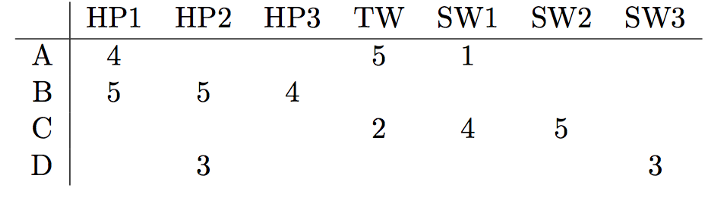
The matrix is extremely sparse. Even after we kept only active users and movies in our experiment below, just 1.4% of the cells were filled. Recommendation is the problem of predicting the values of the empty cells, or at least which empty cells a user would fill in next.

Content-based filtering

Content-based methods recommend items that are similar to the items a user liked before, based on the items’ attributes. For films, the attributes might be genre, director, cast, year and plot description; for news articles, the words they contain; for products, the category, brand and price.

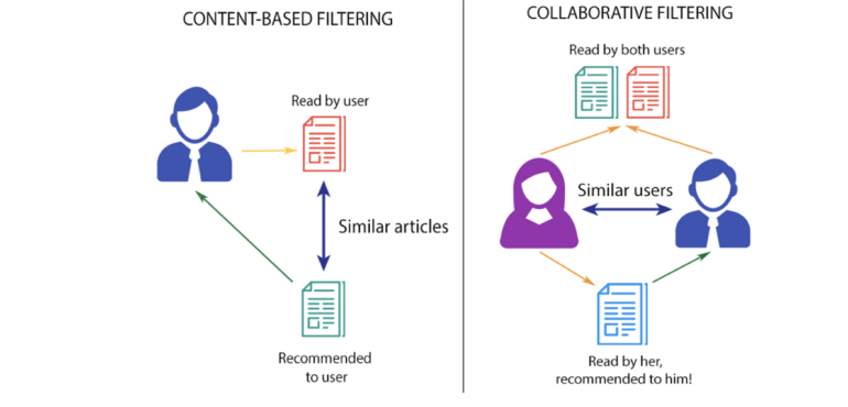
The usual recipe is to turn each item into a vector and each user into a profile built from the items they liked:

• Item vectors can be one-hot encoded attributes, TF-IDF scores of the words in a description (how important a word is for this document compared with the whole collection) or, today, text and image embeddings from a neural network.
• User profiles are often the average of the vectors of the items they interacted with.
• Similarity between vectors is usually measured with cosine similarity, cos(a, b) = a·b / (‖a‖ ‖b‖), which compares the direction of two vectors and works well for high-dimensional data such as text. For binary vectors, Jaccard similarity, the size of the intersection divided by the size of the union, is a simple alternative.

Content-based filtering needs no data about other users, so it can recommend brand-new items as soon as they have a description, and its recommendations are easy to explain (“because you watched another film by this director”). Its weaknesses are over-specialisation, since it rarely surprises users with something outside their usual taste, and the need for good item features. A related approach treats recommendation as an ordinary supervised learning problem: predict whether a user will click or buy from user, item and context features with a model such as gradient boosting. This is how many ranking models in industry work.

Collaborative filtering

Collaborative filtering ignores item attributes and relies only on behaviour. Its assumption: if users A and B liked many of the same things in the past, A will probably like other things B liked. It discovers relationships no attribute describes: people who like a certain cult comedy may also like a certain podcast, for reasons nobody wrote down.

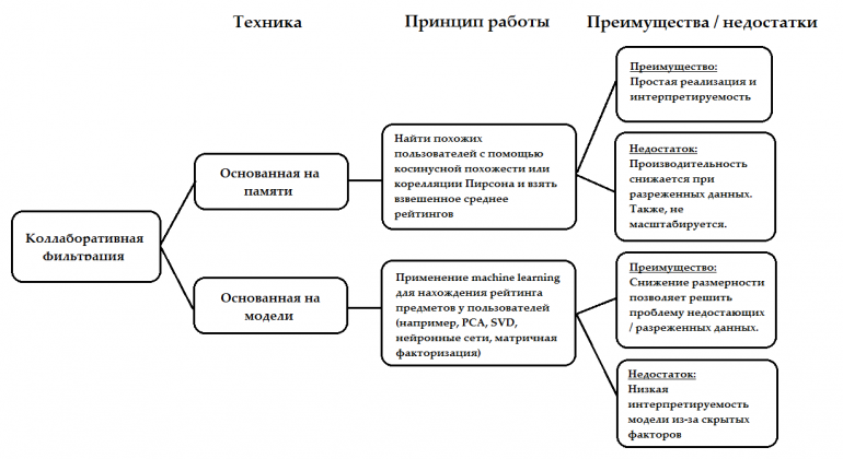
Memory-based: user-based and item-based

User-based collaborative filtering finds the users most similar to you and predicts your rating of an item as a weighted average of their ratings, adjusted for the fact that some people rate everything higher than others. Similarity between users is computed with cosine similarity or the Pearson correlation of their ratings.

Item-based collaborative filtering, introduced at Amazon around 1998 and described in a 2003 paper by Greg Linden, Brent Smith and Jeremy York, turns this around: it finds items that are often liked by the same people, then recommends items similar to those you liked. Item similarities change slowly and can be computed in advance, which made the method practical at Amazon’s scale. “Customers who bought this item also bought” is item-based collaborative filtering.

Memory-based methods are simple and explainable, but they struggle when data is very sparse and when the number of users and items reaches the millions.

Matrix factorization and the Netflix Prize

Model-based methods learn a compact model of the utility matrix. The most influential is matrix factorization: approximate the large, sparse ratings matrix as the product of two thin matrices, one with a vector for each user and one with a vector for each item.

Each user u gets a vector p_u and each item i a vector q_i of, say, 50 numbers called latent factors. The predicted rating is their dot product plus bias terms: r̂_ui = μ + b_u + b_i + p_u·q_i, where μ is the average rating, b_u says how generous the user is and b_i how good the item is in general. The vectors are learned by minimising the squared error on known ratings, with regularisation, using gradient descent or alternating least squares. Nobody tells the model what the factors mean, but they often turn out to capture recognisable dimensions such as “serious drama vs light comedy” or “aimed at children”.

Matrix factorization became famous through the Netflix Prize. In 2006 Netflix offered $1 million to the first team that improved the accuracy of its rating predictions by 10%. In September 2009 the team BellKor’s Pragmatic Chaos won with a 10.06% improvement, using a blend of hundreds of models built around matrix factorization. The competition popularised these methods across the industry, although Netflix itself later moved from predicting star ratings to ranking what people actually watch.

For implicit feedback, where there are no ratings, the same idea is applied to the matrix of interactions: weighted matrix factorization, alternating least squares (ALS) and simple truncated SVD (“PureSVD”) are standard baselines.

Deep learning and generative recommenders

Large platforms rank millions of items for hundreds of millions of users in milliseconds. They do it in stages:

1. Candidate generation (retrieval) narrows millions of items to a few hundred, using cheap methods: item-to-item similarity, matrix factorization or a two-tower model, which encodes users and items with two neural networks into the same vector space so that the nearest items can be found with fast approximate nearest neighbour search.
2. Ranking scores the candidates with a heavier model that uses hundreds of features about the user, item and context: the time of day, device, recent activity. Typical architectures are Google’s Wide & Deep, Meta’s DLRM and gradient-boosted trees, trained to predict clicks, watch time or purchases.
3. Re-ranking adjusts the final list for diversity, freshness, fairness and business rules, so that the home screen is not ten nearly identical items.

Since the late 2010s, sequential recommenders have modelled the order of a user’s actions, first with recurrent neural networks and then with transformers such as SASRec and BERT4Rec: what you watched in the last hour says more about what you want now than what you watched a year ago. Other neural approaches include autoencoders, such as the variational autoencoder for collaborative filtering, and graph neural networks.

The newest wave treats recommendation like language modelling. Generative recommenders predict the next item in a user’s history the way a language model predicts the next word. Meta’s HSTU architecture, presented in 2024, scaled such models to more than a trillion parameters and reported large gains in production. Google’s research on Semantic IDs represents each item as a short sequence of tokens, so a transformer can generate item IDs directly. In 2026 Netflix described GenRec, a ranker built on its own foundation language model that reads user histories and item metadata as text, and tested it on about 10% of its traffic. Large language models are also used for conversational recommendation (“find me a thriller like this, but shorter”) and to generate explanations.

How recommendations are evaluated

Choosing what to optimise is one of the hardest parts of building a recommender: the goal is usually not to recommend what the user already bought or watched. Evaluation happens offline, on historical data, and online, with real users.

Rating accuracy

If the system predicts ratings, compare predictions with real ratings using mean absolute error (MAE, the average absolute difference) or root mean squared error (RMSE, which penalises large errors more). Lower is better. The Netflix Prize was judged on RMSE.

Ranking quality

Most systems show a short list, so it matters whether the right items are near the top:

• Precision@k: the share of the top k recommendations that are relevant.
• Recall@k: the share of all relevant items that appear in the top k.
• Hit rate@k: the share of users for whom at least one relevant item appears in the top k.
• MAP and NDCG: mean average precision and normalised discounted cumulative gain reward placing relevant items higher in the list.

Beyond accuracy

A list of the ten most popular items can score well and still be useless. Teams therefore also track coverage (how much of the catalogue ever gets recommended), diversity within a list, novelty and serendipity (pleasant surprises the user would not have found alone). In the end, every change is tested online with A/B tests on business metrics such as engagement, retention and revenue, because offline metrics often disagree with real user behaviour.

One practical rule: split data by time. If you train on a random 80% of interactions, the model can “see the future” (for example, ratings of a film from after the moment you are predicting), and offline results look better than they will in reality.

Our experiment: five recommenders on real movie ratings

We tested five recommenders on MovieTweetings, an open data set of IMDb ratings (0 to 10) that people posted on Twitter between 2013 and 2021, collected by Simon Dooms and published under the MIT licence. We kept users and movies with at least 20 ratings: 593,400 ratings by 8,576 users of 4,779 movies. For every user, the oldest 80% of their ratings were used for training and the newest 20% became the “future”. The task: recommend 10 movies the user had not rated yet, and count a success when the user later rated a recommended movie 8 or higher.

The five methods: random choice, the ten most popular movies, item-based collaborative filtering with cosine similarity, matrix factorization (truncated SVD with 64 factors) and EASE, a simple linear model published by Harald Steck in 2019 that predicts each movie from all the others and is a strong modern baseline. The code needs only NumPy, pandas and SciPy; download ratings.dat and movies.dat from the MovieTweetings repository on GitHub first.

import numpy as np
import pandas as pd
from scipy.sparse import csr_matrix
from scipy.sparse.linalg import svds

# 1. Data: MovieTweetings, IMDb ratings (0-10) that people posted on Twitter, 2013-2021
r = pd.read_csv("ratings.dat", sep="::", engine="python", names=["user", "movie", "rating", "ts"])
for _ in range(3):                                     # keep users and movies with at least 20 ratings
    r = r[r.groupby("user").movie.transform("size") >= 20]
    r = r[r.groupby("movie").user.transform("size") >= 20]
print(f"{len(r):,} ratings, {r.user.nunique():,} users, {r.movie.nunique():,} movies")

# 2. Time-based split: each user's latest 20% of ratings are the "future" we try to predict
r = r.sort_values("ts")
r["rank"] = r.groupby("user").cumcount() / r.groupby("user").movie.transform("size")
train, test = r[r["rank"] < 0.8], r[r["rank"] >= 0.8]
users = {u: i for i, u in enumerate(r.user.unique())}
movies = {m: i for i, m in enumerate(r.movie.unique())}
X = csr_matrix((np.ones(len(train)), (train.user.map(users), train.movie.map(movies))),
               shape=(len(users), len(movies)))                     # who rated what (1 = rated)
liked = test[test.rating >= 8].groupby("user").movie.apply(lambda s: {movies[m] for m in s})

# 3. Recommenders: each returns a score for every movie for one user
popularity = np.asarray(X.sum(axis=0)).ravel()
norms = np.sqrt(np.asarray(X.multiply(X).sum(axis=0)).ravel()) + 1e-9
item_sim = (X.T @ X).toarray() / np.outer(norms, norms)               # cosine similarity of movies
np.fill_diagonal(item_sim, 0)
U, s, Vt = svds(X.astype(float), k=64)                                # matrix factorization (PureSVD)
G = (X.T @ X).toarray() + 500 * np.eye(len(movies))                   # EASE (Steck, 2019): a linear
P = np.linalg.inv(G)                                                  # model that predicts each movie
B = -P / np.diag(P)                                                   # from all the others
np.fill_diagonal(B, 0)
rng = np.random.default_rng(0)

recommenders = {
    "Random": lambda u: rng.random(len(movies)),
    "Most popular": lambda u: popularity.astype(float),
    "Item-based kNN": lambda u: X[u].toarray().ravel() @ item_sim,
    "Matrix factorization": lambda u: (U[u] * s) @ Vt,
    "EASE": lambda u: X[u].toarray().ravel() @ B,
}

titles = pd.read_csv("movies.dat", sep="::", engine="python", names=["movie", "title", "genres"],
                     encoding="utf-8").set_index("movie").title
ids = list(movies)
for movie in [1375666, 2294629]:                                       # Inception, Frozen
    nearest = np.argsort(-item_sim[movies[movie]])[:5]
    print(f"people who rated {titles[movie]} also rated:", "; ".join(titles[ids[j]] for j in nearest))

# 4. Evaluate top-10 lists: did the user later rate the recommended movies 8 or higher?
print(f"users evaluated: {len(liked):,}")
for name, score in recommenders.items():
    hits, precision, recall, shown = 0, [], [], set()
    for user, relevant in liked.items():
        u = users[user]
        scores = score(u)
        scores[X[u].indices] = -np.inf                                 # never recommend what was already rated
        top10 = np.argpartition(-scores, 10)[:10]
        n = len(relevant & set(top10))
        hits += n > 0
        precision.append(n / 10)
        recall.append(n / len(relevant))
        shown.update(top10)
    print(f"{name:22s} hit rate {hits / len(liked):.3f}  precision@10 {np.mean(precision):.3f}  "
          f"recall@10 {np.mean(recall):.3f}  catalogue coverage {len(shown) / len(movies):.1%}")

593,400 ratings, 8,576 users, 4,779 movies
people who rated Inception (2010) also rated: Forrest Gump (1994); Fight Club (1999); Se7en (1995); The Prestige (2006); The Dark Knight (2008)
people who rated Frozen (2013) also rated: The Hunger Games: Catching Fire (2013); The Hobbit: The Desolation of Smaug (2013); Gravity (2013); The Lego Movie (2014); The Wolf of Wall Street (2013)
users evaluated: 8,263
Random                 hit rate 0.014  precision@10 0.001  recall@10 0.002  catalogue coverage 100.0%
Most popular           hit rate 0.138  precision@10 0.018  recall@10 0.036  catalogue coverage 1.6%
Item-based kNN         hit rate 0.179  precision@10 0.023  recall@10 0.051  catalogue coverage 17.0%
Matrix factorization   hit rate 0.180  precision@10 0.022  recall@10 0.047  catalogue coverage 16.0%
EASE                   hit rate 0.199  precision@10 0.025  recall@10 0.055  catalogue coverage 21.7%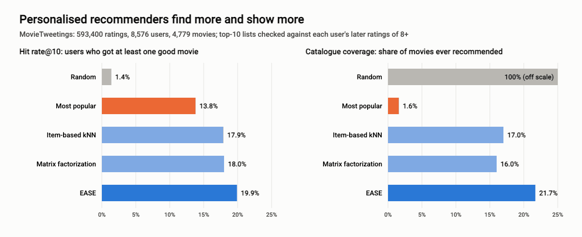

What the numbers show:

• Personalisation works. For 19.9% of users, EASE put at least one movie they later rated highly into a top-10 list chosen from 4,779 movies, against 13.8% for the popularity list and 1.4% for random choice. EASE beats popularity by 44% on hit rate and by 53% on recall@10.
• Popularity is a strong but narrow baseline. It shows everyone the same 10 movies, covering just 1.6% of the catalogue. The personalised methods recommended 16% to 22% of all movies at least once, so many more films get a chance to be discovered.
• Simple methods are close. Item-based kNN and matrix factorization performed almost identically. The best model is not always the most complex one, which is why simple baselines like EASE and item-kNN are still used in research to check claims about deep models.
• The task is hard. Precision@10 of 2.5% sounds low, but predicting which of almost 5,000 films a person will rate highly is difficult: each user’s “future” can stretch over months or years of changing tastes, and a top-10 list is a very small window.

The lists of similar movies show how collaborative filtering thinks. The neighbours of Inception are films that the same audience loved: The Prestige, The Dark Knight, Fight Club. The neighbours of Frozen are other 2013 blockbusters such as Catching Fire and The Desolation of Smaug, not other animated films, because collaborative filtering captures who watched things and when, not what they are about. Hybrid systems combine both kinds of signal for exactly this reason.

Challenges: cold start, bias and filter bubbles

• Cold start. A new user has no history and a new item has no interactions, so collaborative filtering cannot help. Systems fall back on popularity, ask new users a few onboarding questions, and use content features or embeddings of new items until behaviour data arrives.
• Popularity bias and feedback loops. Items that are recommended get more clicks, which makes them look better and get recommended even more. Without countermeasures, the catalogue’s long tail is never seen. Exploration, for example with multi-armed bandits that occasionally show less certain items, helps break the loop.
• Filter bubbles. Optimising only for engagement can narrow what people see and amplify sensational content. Diversity constraints in re-ranking and long-term satisfaction metrics address this. In the EU, the Digital Services Act requires very large online platforms to explain the main parameters of their recommender systems and to offer at least one option that is not based on profiling.
• Scale and latency. Recommendations must be computed for millions of users in tens of milliseconds, which shapes the whole architecture: precomputed embeddings, approximate nearest neighbour search and caching.
• Privacy. Recommenders rely on detailed behaviour data, which requires consent, data minimisation and, increasingly, techniques such as on-device or federated learning.

How to build a recommender system

1. Define the goal and the metric. What should users do more of: watch, buy, return? Choose an offline metric that tracks it and plan an A/B test.
2. Collect interaction data with timestamps, plus item metadata. Log what was shown as well as what was clicked, so you can learn from items that were ignored.
3. Start with baselines: most popular, recently popular, item-to-item similarity. They are quick to build and surprisingly hard to beat.
4. Add a learned model: matrix factorization or EASE for collaborative filtering, gradient-boosted trees for ranking with features, then neural two-tower and sequential models when data and traffic justify them. Neural models train on GPUs; see our guide to the best GPU for AI.
5. Evaluate with time-based splits, track coverage and diversity as well as accuracy, then test online.

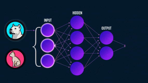
Useful open-source libraries include implicit (fast ALS and nearest neighbour models for implicit feedback), LightFM (hybrid matrix factorization with features), RecBole (more than 90 algorithms behind one interface, useful for research), Microsoft’s Recommenders (examples and best practices), Meta’s TorchRec and NVIDIA Merlin for large-scale deep learning recommenders. The models are trained like any neural network, with backpropagation; our PyTorch vs TensorFlow comparison helps choose a framework.

FAQ

What are the main types of recommender systems?

Content-based filtering recommends items similar to those a user liked, based on item attributes. Collaborative filtering recommends items liked by similar users, based only on behaviour. Hybrid systems combine both, and most production systems are hybrids built with machine learning and deep learning models.

How does the Netflix recommendation algorithm work?

Netflix uses many models rather than one algorithm: they personalise which rows appear on the home page, the order of titles in each row, the artwork shown for each title and search results. They learn from viewing history, ratings, time of day and device. In 2026 Netflix described a ranker built on its own foundation language model that it tested on part of its traffic.

What is the difference between collaborative filtering and content-based filtering?

Content-based filtering looks at what items are (genre, words, features) and needs only the user’s own history. Collaborative filtering looks at who interacted with items and needs data from many users, but can discover connections that item features do not show. Collaborative filtering struggles with new items; content-based filtering struggles to surprise users.

What is the cold start problem?

It is the difficulty of recommending to new users who have no history, or recommending new items that nobody has interacted with yet. Common fixes are popularity-based defaults, onboarding questions and content-based features until enough behaviour data is collected.

Which algorithm is best for a recommender system?

There is no single best one. Strong, simple baselines such as item-based collaborative filtering, matrix factorization and EASE should come first, as our experiment shows; large platforms add gradient-boosted or neural ranking models and, increasingly, transformer-based sequential and generative recommenders. The right choice depends on the amount of data, the importance of new items, latency limits and the business goal.

Are recommendation systems machine learning?

Yes. Apart from hand-made rules such as “show the newest items”, recommender systems learn from data about user behaviour and item properties, which makes them one of the most widely used applications of machine learning.