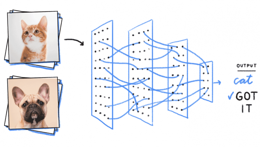
A perceptron is the simplest neural network: a single artificial neuron that takes several inputs, multiplies each by a weight, adds them up with a bias and outputs 1 or 0 depending on whether the sum crosses a threshold. It is a binary classifier that separates two classes with a straight line, or a flat plane in more dimensions, and it comes with a remarkably simple learning rule. Invented by Frank Rosenblatt in 1957, the perceptron was the first machine that could learn from examples. Its limits, made famous by the XOR problem, contributed to the first “AI winter”, and stacking perceptrons into layers, the multilayer perceptron, became the foundation of modern deep learning.
This guide covers the history of the perceptron, how it works, the perceptron learning algorithm with a Python implementation from scratch, why a single perceptron cannot learn XOR and how a two-layer network solves it, and the multilayer perceptron, with code and results.
Key takeaways
- Model:
y = step(w · x + b), a weighted sum of the inputs plus a bias, passed through a step function. - Learning rule: after each mistake,
w ← w + η (target − prediction) x. If the classes can be separated by a straight line, the algorithm is guaranteed to find one. - Limitation: a single perceptron is a linear classifier, so it cannot solve problems like XOR whose classes are not linearly separable.
- Multilayer perceptron (MLP): layers of neurons with non-linear activations, trained with backpropagation, can approximate any continuous function.
- Today: every neural network is built from perceptron-like units, and MLP blocks hold most of the parameters of Transformers.
What Is a Perceptron?
A perceptron is an algorithm for binary classification: it decides whether an input belongs to one category or the other, for example whether a picture shows a cat or not, or whether an email is spam. It is a linear classifier, which means it makes its decision with a linear function of the inputs: it draws a straight line, or in many dimensions a hyperplane, and puts everything on one side into class 1 and everything on the other side into class 0.
The perceptron is loosely modeled on a biological neuron. The inputs play the role of dendrites, the weights of synaptic strengths, and the output of the axon that either fires or stays silent. It is the basic unit from which larger neural networks are built, which is why the term is also used for a single artificial neuron in general.
Rosenblatt’s Perceptron: the Machine That Learned
The idea of an artificial neuron goes back to Warren McCulloch and Walter Pitts, who in 1943 described a neuron as a logical threshold unit: it fires if the sum of its binary inputs exceeds a threshold. Their neurons could compute logical functions, but their weights had to be set by hand. What was missing was a way to learn them.
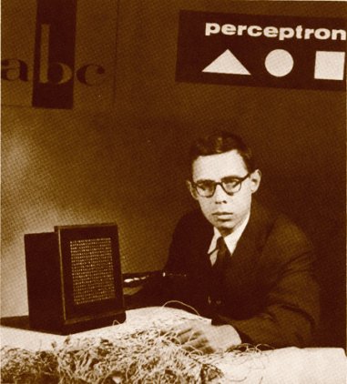
Frank Rosenblatt, a psychologist at the Cornell Aeronautical Laboratory, supplied it. In 1957 he described the perceptron and a rule for adjusting its weights from examples, and with funding from the US Office of Naval Research he built it as a machine rather than a program. The Mark I Perceptron, completed around 1960, had a camera of 400 photocells arranged in a 20 × 20 grid connected to “association units”, and its weights were potentiometers turned by electric motors during learning. It could learn to tell simple shapes and letters apart.
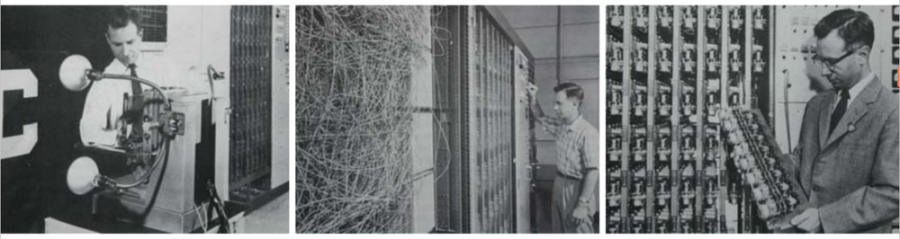
The perceptron caused a sensation. Press reports in 1958 predicted machines that would soon walk, talk, see and be aware of their own existence. Then, in 1969, Marvin Minsky and Seymour Papert published the book Perceptrons, which proved mathematically what single-layer perceptrons cannot do, most famously compute the XOR function. The book was widely read as a verdict on neural networks in general, funding moved to symbolic AI, and neural network research went through a long decline often called the first AI winter. Rosenblatt died in a boating accident in 1971.
The way out was known in principle: networks with several layers of neurons could compute XOR and much more. What was missing was an efficient way to train them. It came with the popularization of backpropagation by David Rumelhart, Geoffrey Hinton and Ronald Williams in 1986, and the deep learning revolution of the 2000s and 2010s, led by Hinton and others, finally fulfilled much of what the perceptron had promised. The Mark I Perceptron is now in the Smithsonian’s National Museum of American History.
How a Perceptron Works
A perceptron takes an input vector x = (x1, …, xn), multiplies each input by its weight, adds a bias b and applies an activation function φ:
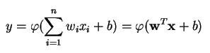
Here w is the weight vector, x the input vector, b the bias and φ the activation. In the classic perceptron, φ is the step function: it outputs 1 if w · x + b ≥ 0 and 0 otherwise. The weights say how important each input is and whether it pushes the decision towards 1 or towards 0; the bias shifts the threshold, so the neuron can fire even when all inputs are zero or stay silent when they are large.
Geometrically, the equation w · x + b = 0 defines a straight line in two dimensions, a plane in three and a hyperplane in general. This is the decision boundary. The weight vector is perpendicular to it, and the bias moves it away from the origin. Everything on one side is classified as 1, everything on the other side as 0. That is the source of both the perceptron’s simplicity and its main limitation.
For example, a perceptron with weights (1, 1) and bias −1.5 computes logical AND of two binary inputs: the sum crosses zero only when both inputs are 1. With bias −0.5 it computes OR.
The Perceptron Learning Algorithm
Rosenblatt’s learning rule is one of the simplest in machine learning. It is a form of supervised learning: the perceptron is trained on examples with known labels.
- Start with weights and bias equal to zero (or small random numbers).
- Take a training example
xwith labely(0 or 1) and compute the predictionŷ = step(w · x + b). - If the prediction is correct, do nothing. If it is wrong, update the weights and bias:
w ← w + η (y − ŷ) x,b ← b + η (y − ŷ),
whereηis the learning rate. - Repeat over the training set, epoch after epoch, until an entire pass produces no mistakes or a maximum number of epochs is reached.
The update has an intuitive meaning. If the perceptron outputs 0 for an example of class 1, y − ŷ = 1, and the input is added to the weights, which increases w · x for this example next time. If it outputs 1 for class 0, the input is subtracted. Each mistake turns the decision boundary towards the misclassified point.
The perceptron convergence theorem, proved by Albert Novikoff in 1962, guarantees that if the two classes can be separated by a hyperplane, the algorithm finds one after a finite number of mistakes. The number of mistakes is at most (R / γ)2, where R is the largest distance of a training point from the origin and γ is the margin, the distance from the separating hyperplane to the nearest point. A wide margin means fast learning. If the classes are not linearly separable, the algorithm never settles and the weights keep changing forever.
Perceptron in Python from Scratch
Here is the whole algorithm in a few lines of NumPy, trained on three logical functions of two binary inputs:
import numpy as np

class Perceptron:
    def __init__(self, lr=1.0, epochs=100):
        self.lr, self.epochs = lr, epochs

    def predict(self, X):
        return np.where(X @ self.w + self.b >= 0, 1, 0)        # step activation

    def fit(self, X, y):
        self.w, self.b = np.zeros(X.shape[1]), 0.0
        for epoch in range(1, self.epochs + 1):
            mistakes = 0
            for xi, target in zip(X, y):
                error = target - self.predict(xi)                # +1, 0 or -1
                if error != 0:                                   # update only on mistakes
                    self.w += self.lr * error * xi
                    self.b += self.lr * error
                    mistakes += 1
            if mistakes == 0:                                    # every example is classified correctly
                print(f"  converged after {epoch} epochs")
                return self
        print(f"  no convergence after {self.epochs} epochs")
        return self

X = np.array([[0, 0], [0, 1], [1, 0], [1, 1]])
for name, y in [("AND", [0, 0, 0, 1]), ("OR", [0, 1, 1, 1]), ("XOR", [0, 1, 1, 0])]:
    print(name)
    p = Perceptron().fit(X, np.array(y))
    print(f"  weights {p.w}, bias {p.b}, predictions {p.predict(X)}, targets {y}")
AND
converged after 6 epochs
weights [2. 1.], bias -3.0, predictions [0 0 0 1], targets [0, 0, 0, 1]
OR
converged after 4 epochs
weights [1. 1.], bias -1.0, predictions [0 1 1 1], targets [0, 1, 1, 1]
XOR
no convergence after 100 epochs
weights [-1. 0.], bias 0.0, predictions [1 1 0 0], targets [0, 1, 1, 0]The perceptron learns AND in six epochs and OR in four. The weights it finds are different from the ones we chose by hand above, but any line that separates the classes is a valid solution. For XOR it never converges: after 100 epochs the weights are still jumping around and only two of the four examples are classified correctly. In practice you can use scikit-learn’s Perceptron class, which implements the same algorithm with extras such as shuffling and regularization.
The XOR Problem
XOR, “exclusive or”, outputs 1 when exactly one of its two inputs is 1. Plot the four inputs on a plane and the problem becomes obvious: the points (0, 1) and (1, 0) of class 1 sit on one diagonal of a square, (0, 0) and (1, 1) of class 0 on the other. No single straight line can put both 1s on one side and both 0s on the other. The classes are not linearly separable, and since a perceptron can only draw straight lines, it cannot represent XOR at all, whatever its weights.
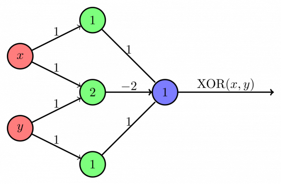
A network with a hidden layer can. In the network below, the hidden neurons compute simple threshold functions of the inputs: the top one fires when x is 1, the middle one when both inputs are 1 (threshold 2), and the bottom one when y is 1. The output neuron adds the outer two and subtracts twice the middle one, so it fires when exactly one input is on:
import numpy as np

step = lambda z: (z >= 0).astype(int)

def xor_network(x, y):
    h1 = step(x - 1)               # fires if x = 1           (threshold 1)
    h2 = step(x + y - 2)           # fires if x = 1 and y = 1 (threshold 2)
    h3 = step(y - 1)               # fires if y = 1           (threshold 1)
    return step(h1 - 2 * h2 + h3 - 1)

for x, y in [(0, 0), (0, 1), (1, 0), (1, 1)]:
    print(x, y, "->", xor_network(np.array(x), np.array(y)))
0 0 -> 0
0 1 -> 1
1 0 -> 1
1 1 -> 0The hidden layer transforms the inputs into a new representation in which the problem becomes linearly separable for the output neuron. That is the key idea of multilayer networks. Minsky and Papert knew that multilayer networks could compute XOR; the open question at the time was how to learn their weights automatically instead of designing them by hand.
The Multilayer Perceptron
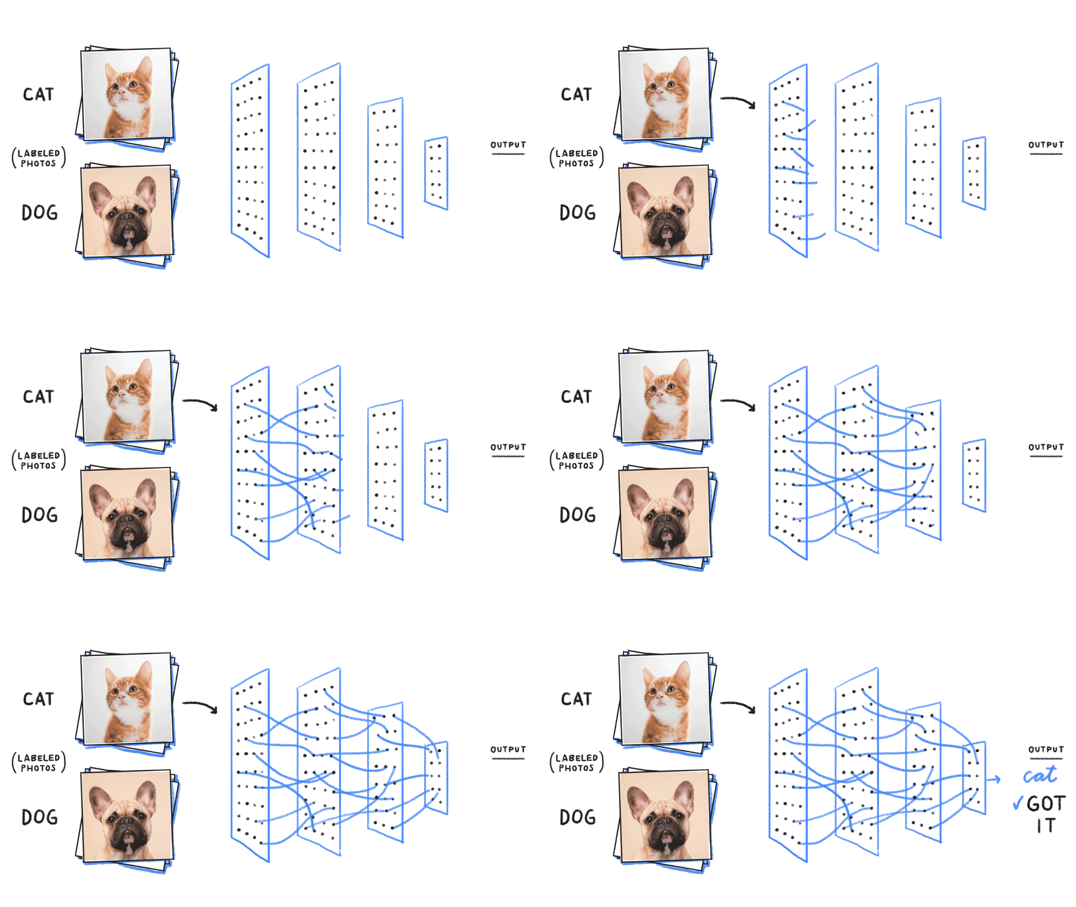
A multilayer perceptron (MLP) is a feedforward neural network made of several layers of neurons. It has an input layer that receives the data, one or more hidden layers that do the real computation, and an output layer that makes the prediction. Every neuron in a layer is connected to every neuron in the next one, which is why these layers are also called fully connected or dense layers.
Two changes make MLPs trainable and powerful:
- Smooth non-linear activations. The step function has zero gradient almost everywhere, so it gives no signal about how to change the weights. MLPs use differentiable activation functions such as sigmoid, tanh or ReLU. Without a non-linearity, any stack of layers would collapse into a single linear function, no more powerful than one perceptron.
- Backpropagation. Training works like a game of ping-pong. In the forward pass, the input flows through the layers and the output is compared with the correct answer, producing a loss, for example cross-entropy or mean squared error. In the backward pass, the chain rule sends the gradient of the loss back through the network to every weight and bias, and an optimizer such as stochastic gradient descent or Adam updates them. The process repeats until the error stops decreasing, and the network is said to have converged.
The universal approximation theorem, proved by George Cybenko in 1989 and Kurt Hornik in 1991, shows that an MLP with a single hidden layer and enough neurons can approximate any continuous function on a bounded domain as closely as desired. The theorem says nothing about how many neurons are needed or whether training will find the right weights; in practice deeper networks with several hidden layers learn more efficiently than one huge layer.
Here is the difference in practice on a dataset that a straight line cannot separate: two interleaving half-circles, the “two moons”:
from sklearn.datasets import make_moons
from sklearn.model_selection import train_test_split
from sklearn.linear_model import Perceptron
from sklearn.neural_network import MLPClassifier

X, y = make_moons(n_samples=1000, noise=0.2, random_state=0)   # two interleaving half-circles
X_train, X_test, y_train, y_test = train_test_split(X, y, test_size=0.3, random_state=0)

perceptron = Perceptron(random_state=0).fit(X_train, y_train)
mlp = MLPClassifier(hidden_layer_sizes=(16, 16), max_iter=2000, random_state=0).fit(X_train, y_train)

print(f"single-layer perceptron: test accuracy {perceptron.score(X_test, y_test):.3f}")
print(f"multilayer perceptron:   test accuracy {mlp.score(X_test, y_test):.3f}")
print("MLP layer sizes:", [w.shape for w in mlp.coefs_])
print("MLP parameters:", sum(w.size for w in mlp.coefs_) + sum(b.size for b in mlp.intercepts_))
single-layer perceptron: test accuracy 0.830
multilayer perceptron: test accuracy 0.953
MLP layer sizes: [(2, 16), (16, 16), (16, 1)]
MLP parameters: 337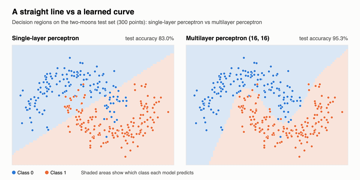
The perceptron does what it can with one straight line and gets 83% of the test points right. The MLP with two hidden layers of 16 ReLU neurons, 337 parameters in total, bends its decision boundary around the moons and reaches 95.3%. The remaining errors are mostly points that the noise has pushed deep into the other class’s territory.
Perceptron vs Logistic Regression vs MLP
| Perceptron | Logistic regression | Multilayer perceptron | |
|---|---|---|---|
| Decision boundary | Linear | Linear | Non-linear |
| Activation | Step | Sigmoid | ReLU, tanh, sigmoid in hidden layers |
| Output | Class label 0 or 1 | Probability | Probabilities or numbers |
| Training | Perceptron rule, updates only on mistakes | Gradient descent on log loss | Backpropagation and gradient descent |
| Non-separable data | Never converges | Finds the best linear fit | Can fit complex boundaries |
| Typical use | Teaching, simple online learning | Interpretable baseline classifier | Tabular data, building block of deep networks |
Logistic regression is the perceptron’s smoother sibling: the same weighted sum, but with a sigmoid instead of a step, which turns the output into a probability and makes the loss differentiable. A neuron in an MLP is a perceptron with a differentiable activation; with a single neuron and a sigmoid output, an MLP becomes logistic regression. For regression tasks, a single neuron with no activation is linear regression.
Perceptrons in Modern Deep Learning
The single-layer perceptron is rarely used on its own today, but its descendants are everywhere. Every layer of a deep network is a set of perceptron-like units computing weighted sums followed by non-linearities. Convolutional networks apply such neurons to small patches of an image, recurrent networks to sequences, and they usually end with an MLP classifier.
The Transformers behind modern language models alternate attention layers with MLP blocks, often called feed-forward layers, and these MLP blocks hold about two-thirds of the parameters of a typical model. Research keeps revisiting the idea: MLP-Mixer (2021) showed that an architecture built only from MLPs can compete on image classification, and Kolmogorov-Arnold Networks (2024) proposed replacing fixed activations on neurons with learnable functions on the connections. On tabular data, a well-tuned MLP remains a strong baseline, although gradient boosting often still wins.
FAQ
What is a perceptron in simple terms?
It is a single artificial neuron that makes a yes-or-no decision. It weighs its inputs, adds them up, and outputs 1 if the total is above a threshold and 0 otherwise. Training adjusts the weights each time it makes a mistake.
Who invented the perceptron?
Frank Rosenblatt, a psychologist at the Cornell Aeronautical Laboratory, in 1957. He built the Mark I Perceptron, a hardware machine with 400 photocells, around 1960. It was based on the artificial neuron of McCulloch and Pitts from 1943.
What is the difference between a perceptron and a neuron?
In machine learning the words are often used interchangeably. Strictly, the perceptron is a neuron with a step activation and Rosenblatt’s learning rule, while a neuron in a modern network uses a differentiable activation, such as ReLU or sigmoid, and is trained with backpropagation.
Why can’t a perceptron solve XOR?
Because a perceptron separates classes with a straight line, and the XOR classes cannot be separated by any straight line: the two positive points lie on one diagonal of a square and the two negative points on the other. A network with one hidden layer can solve it.
What is the difference between a single-layer and a multilayer perceptron?
A single-layer perceptron connects the inputs directly to the output and can only learn linear decision boundaries. A multilayer perceptron adds hidden layers with non-linear activations and is trained with backpropagation, which lets it learn complex, non-linear functions.
Is the perceptron supervised or unsupervised?
Supervised. It learns from labeled examples and updates its weights whenever its prediction differs from the correct label.
Is an MLP deep learning?
An MLP with several hidden layers is a deep neural network, and MLPs are a core part of deep learning. Deep learning also includes architectures such as CNNs, RNNs and Transformers, all of which contain MLP-like layers.
See also: our guides to backpropagation, the algorithm that made multilayer perceptrons trainable, and to activation functions, which give MLPs their non-linearity.