Mobile Laser Scanning (MLS) systems can now scan large areas, like cities or even countries. The produced 3D point clouds can be used as maps for autonomous systems. To do so, the automatic classification of the data is necessary and is still challenging, regards to the number of objects present in an urban scene. Xavier Roynard, Jean-Emmanuel Deschaud and François Goulette propose both a training method that balances the number of points per class during each epoch and a 3D CNN capable of effectively learning how to classify scenes containing objects at multiple scales.
MS Voxel Deep Network — A new convolutional neural network (CNN) to classify 3D point clouds of urban or indoor scenes. On the reduced-8 Semantic3D benchmark, this network ranked second, beats the state of the art of point classification methods (those not using a regularization step).
Network Learning Difficulties
Training on scenes point cloud leads to some difficulties. For the point classification task, each point is a sample, so the number of samples per class is very unbalanced (from thousands of points for the class “pedestrian” to tens of millions for the class “ground”). Also with the training method of deep-learning, an Epoch would be to pass through all points of the cloud, which would take a lot of time. Indeed, two very close points have the same neighbourhood, and will, therefore, be classified in the same way.
Authors propose a training method that solves these two problems. We randomly select N (for example 1000) points in each class, then we train on these points mixed randomly between classes, and we renew this mechanism at the beginning of each Epoch.
Once a point p to classify is chosen, we compute a grid of voxels given to the convolutional network by building an occupancy grid centered on p whose empty voxels contain 0 and occupied voxels contain 1. We only use NxNxN cubic grids where n is pair, and we only use isotropic space discretization steps ∆.
Network Training
Some classic data augmentation steps are performed before projecting the 3D point clouds into the voxels grid:
• Flip x and y axis, with probability 0.5
• Random rotation around z-axis
• Random scale, between 95% and 105%
• Random occlusions (randomly removing points), up to 5%
• Random artefacts (randomly inserting points), up to 5%
Random noise in position of points, the noise follows a normal distribution centered in 0 with standard deviation 0.01m
The cost function used is cross-entropy, and the optimizer used is ADAM with a learning rate of 0.001 and ε = 10−8, which are the default settings in most deep-learning libraries.
Architecture — Layers
3D Essential Layers
- Conv(n, k, s, p) a convolutional layer that transforms feature maps from the previous layer into n new feature maps, with a kernel of size k × k × k and stride s and pads p on each side of the grid.
- DeConv(n, k, s, p) a transposed convolutional layer that transforms feature maps from the previous layer into n new feature maps, with a kernel of size k × k × k and stride s and pads p on each side of the grid.
- FC(n) a fully-connected layer that transforms the feature maps from the previous layer into n feature maps.
- MaxPool(k) a layer that aggregates on each feature map every group of 8 neighbouring voxels.
- MaxU nPool(k) a layer that computes an inverse of MaxPool(k).
- ReLU, LeakyReLU and PReLU common non-linearities used after linear layers as Conv and FC. ReLU (x) returns the positive part of x, and to avoid null gradient if x is negative, we can add a slight slope which is fixed (LeakyReLU ) or can be learned (PReLU ).
- SoftMax a non-linearity layer that rescales a tensor in the range [0, 1] with sum
- BatchNorm a layer that normalizes samples over a batch.
- DropOut(p) a layer that randomly zeroes some of the elements of the input tensor with probability p.
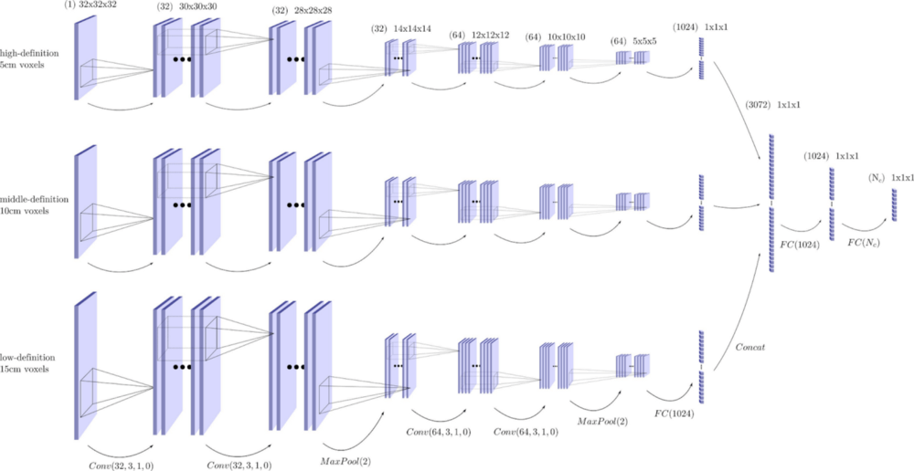
The chosen network architecture is inspired from this one that works well in 2D.
Datasets
Authors compared 3 different datasets. Paris-Lille-3D contains 50 classes but for our experimentations, we keep only 9 coarser classes. In brackets is indicated the number of points after subsampling at 2 cm.
Among the 3D point cloud scenes datasets, these are those with the most area covered and the most variability
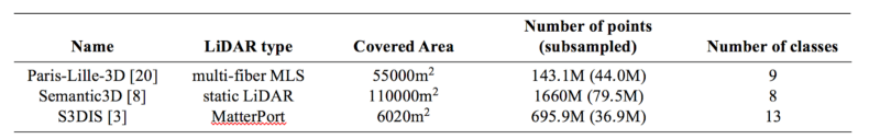
The covered area is obtained by projecting each cloud on a horizontal plane in pixels of size 10cm × 10cm, then summing the area of all occupied pixels.
A finer resolution of 5 cm was added to better capture the local surface near the point, and a coarser resolution of 15 cm to better understand the context of the object to which the point belongs. This method achieves better results than all methods that classify cloud by points (i. e. without regularization). Even better results could probably be achieved by adding, for example, a CRF after classification.
Example of classified point cloud on S3DIS dataset:
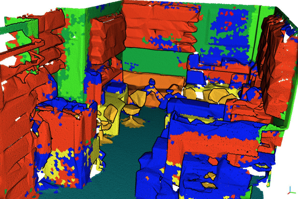
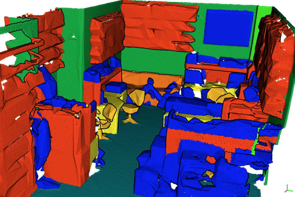
Results are very close to the truth. This is achieved by both focusing on the local shape of the object around a point and by taking into account the context of the object.
Quote:
We observe a confusion between the classes wall and board (and more slightly with beam, column, window and door), this is explained mainly because these classes are very similar geometrically and we do not use color. To improve these results, we should not sub-sample the clouds to keep the geometric information thin (such as the table slightly protruding from the wall) and add a 2 cm scale in input to the network, but looking for neighborhoods would then take an unacceptable amount of time.
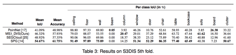
For a comparison with the state-of-the-art methods on S3DIS 5th fold see table below:
To evaluate architecture choices, this classification task was tested by one of the first 3D convolutional networks: VoxNet.
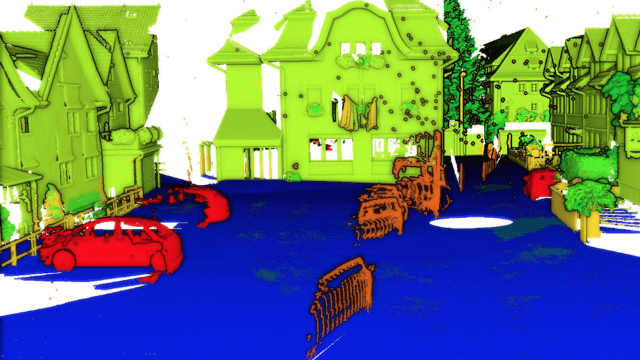
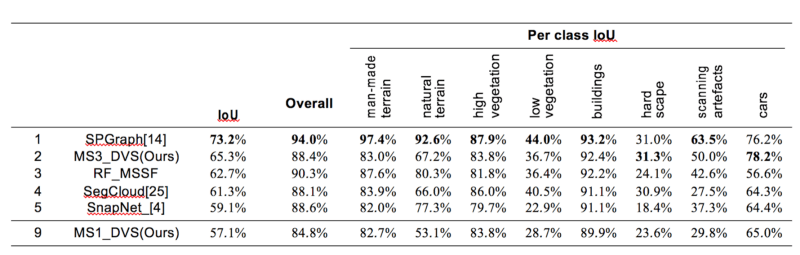
Comparison with the state-of-the-art methods on reduced-8 Semantic3D benchmark:
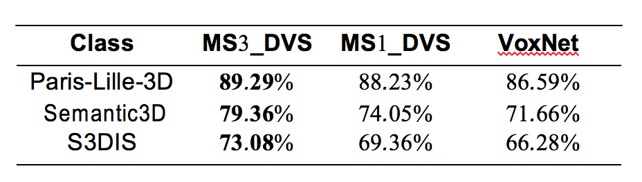
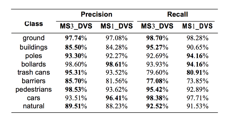
Comparison per class between MS1_DeepVoxScene and MS3_DeepVoxScene on Paris-Lille-3D dataset. This shows that the use of multi-scale networks improves the results on some classes, in particular the buildings, barriers and pedestrians classes are greatly improved (especially in Recall), while the car class loses a lot of Precision.
Conclusion
Proposed training method — MS3_DVS, balances the number of points per class seen during each epoch, as well as a multi-scale CNN that is capable of learning to classify point cloud scenes. You may follow this on Semantic3D benchmark. Now it’s number 2 among all — very good result. This is achieved by both focusing on the local shape of the object around a point and by taking into account the context of the object.