The curse of dimensionality is the name for a group of problems that appear when data has many dimensions, that is, many features or variables. As the number of dimensions grows, the volume of the space grows so fast that any realistic amount of data becomes sparse, distances between points lose their meaning, and methods that work well in two or three dimensions quietly break down. The term was coined by the mathematician Richard Bellman in the late 1950s, and it is one of the most important ideas to understand before training a machine learning model.
This guide explains what the curse of dimensionality is, the strange geometry behind it, how it hurts nearest-neighbour methods, clustering, overfitting and hyperparameter search, why deep neural networks with billions of parameters still manage to learn, and what to do about it. We measured each effect in Python: how distances concentrate in 10,000 dimensions, where the volume of a cube goes, and how a k-nearest neighbours classifier collapses from 94% to 27% accuracy when we add random features to a real data set.
Key takeaways
- The curse of dimensionality: the amount of data needed to cover a space grows exponentially with the number of dimensions. With 10 values per axis, 2 features need 100 combinations, 20 features need 1020.
- Distances concentrate. In our test with 1,000 random points, the farthest point was 135 times farther than the nearest in 2 dimensions, but only 1.11 times farther in 1,000 dimensions. “Nearest neighbour” stops meaning much.
- Irrelevant features hurt distance-based models most. Adding 4,096 random features dropped k-NN accuracy on handwritten digits from 94.4% to 27.2%; a random forest kept 88.0%, and k-NN after feature selection stayed at 95.9%.
- Real data is rarely as high-dimensional as it looks. Images, text and sound lie near low-dimensional structures, which is why neural networks, trained with gradient descent rather than search, can learn from them, and why semantic search over 3,072-dimensional embeddings works.
- Remedies: feature selection, dimensionality reduction (PCA, embeddings), regularization, more data, models with built-in structure, and random rather than grid search for hyperparameters.
What is the curse of dimensionality?
A dimension is one coordinate needed to describe a data point. A house described by area and price is a point in 2 dimensions; a customer described by 300 attributes is a point in 300 dimensions; an 8 × 8 grayscale image is a point in 64 dimensions, and a 1024 × 1024 color photo is a point in more than 3 million dimensions.
The curse of dimensionality refers to the fact that many things become exponentially harder as the number of dimensions grows: covering the space with data, searching it, estimating densities and comparing points by distance. Bellman ran into it in dynamic programming, where dividing each of d variables into 10 levels gives 10d states to evaluate. In machine learning it usually shows up in three ways:
- Data sparsity. To keep the same density of examples, the number of samples must grow exponentially with the number of features. With a fixed data set, every new feature spreads the same points over a much larger space.
- Distance concentration. All points become almost equally far from each other, so methods based on distances or neighbourhoods lose their footing.
- Overfitting. With many features and few examples, a model can find patterns that fit the training data perfectly by chance.
Why high-dimensional space is strange
Our intuition was built in three dimensions, and it fails in high-dimensional space. Four facts, each of which we computed in the experiment below, explain most of the curse.
1. The number of regions explodes
Divide each axis into 10 intervals. In 1 dimension there are 10 cells, in 2 dimensions 100, in 3 dimensions 1,000, in 10 dimensions 10 billion and in 100 dimensions 10100, more than the number of atoms in the observable universe, which is estimated at about 1080. A data set of a million points leaves almost every cell empty. Any method that needs examples “near” every possible input, such as a lookup table, a histogram or a grid search, becomes impossible.
2. The volume moves to the corners and the surface
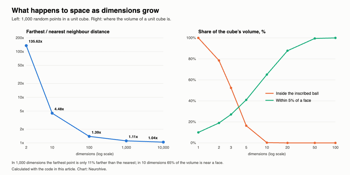
Put a ball inside a unit cube so that it touches every face. In 2 dimensions the circle covers 78.5% of the square; in 3 dimensions the ball covers 52.4% of the cube; in 10 dimensions only 0.25%; in 20 dimensions 0.0000025%. Almost all of the volume of a high-dimensional cube lies in its corners, far from the center.
At the same time, the volume concentrates near the surface. The share of a unit cube that lies within 5% of a face, that is, outside the inner cube of side 0.9, is 1 − 0.9d: 19% in 2 dimensions, 65% in 10 and 99.5% in 50. In high dimensions, almost every random point is an “edge case”.
3. Distances concentrate
In 1999, Beyer, Goldstein, Ramakrishnan and Shaft showed in “When is nearest neighbor meaningful?” that, for broad classes of data, the ratio between the distance to the farthest point and the distance to the nearest point approaches 1 as the number of dimensions grows. Intuitively, the distance is a sum over many coordinates, and sums of many random terms all end up close to their average. Our simulation with 1,000 uniform random points shows it clearly: the farthest point is 135.6 times farther than the nearest in 2 dimensions, 4.5 times in 10, 1.39 times in 100, 1.11 times in 1,000 and 1.04 times in 10,000.
4. Random directions are almost orthogonal
Two random vectors in high dimensions are almost always nearly perpendicular: the cosine of the angle between them is close to 0. This is why random projections work (see below), and also why cosine similarity between unrelated items is near zero in embedding spaces.
How it affects machine learning
- Nearest-neighbour methods and clustering. k-nearest neighbours, k-means, DBSCAN and kernel methods with a distance-based kernel rely on “close” meaning “similar”. When distances concentrate and irrelevant features add noise to every distance, the neighbours found are no longer the right ones. This is the classic curse of dimensionality for k-NN.
- The Hughes phenomenon. In 1968, Gordon Hughes showed that with a fixed number of training examples, adding features first improves a classifier and then makes it worse. Each new feature adds information but also parameters to estimate, and past some point the estimation error wins. This is also called the peaking phenomenon.
- Overfitting. When the number of features approaches or exceeds the number of examples, as in genomics (tens of thousands of genes, hundreds of patients) or text with large vocabularies, a model such as linear regression can fit the training data perfectly and generalize badly unless it is regularized.
- Density estimation and anomaly detection. Estimating a probability density with histograms or kernel density estimation needs exponentially many samples; in high dimensions, every point looks like an outlier.
- Hyperparameter search. A grid with 5 values for each of 6 hyperparameters has 15,625 combinations. Bergstra and Bengio showed in 2012 that random search finds good settings much faster than grid search, because usually only a few hyperparameters matter, and a grid wastes most trials on the unimportant ones.
Neural networks: why searching for weights fails
Training a neural network means finding the set of weights that minimizes the error, and the network’s weights form a space with one dimension per weight. The weights depend on each other: a small change of one weight in the first layer changes the signal that every later layer receives, so the weights cannot be tuned one at a time.
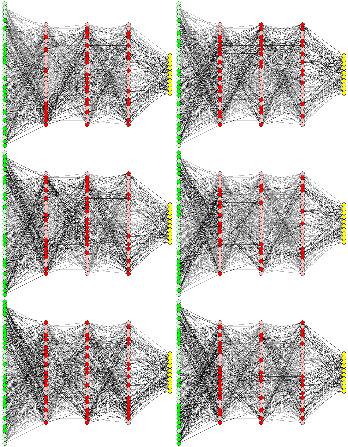
The most naive approach would be to try many random sets of weights, or a grid of them, and keep the best. For a tiny network with 2 weights, 10 values per weight give 100 combinations and 100 values per weight give 10,000, which a computer checks in a fraction of a second. For 3 weights it is 1,000 or 1,000,000. But a small network for the MNIST handwritten digits, with 784 inputs, 15 hidden neurons and 10 outputs, already has 784 × 15 + 15 × 10 = 11,910 weights. A grid with 10 values per weight would have 1011,910 points, compared with roughly 1080 atoms in the observable universe. Modern language models have billions or trillions of weights.
That is why neural networks are not trained by search, but by gradient descent: backpropagation computes, in one pass, the direction in which every weight should change to reduce the error, and the network takes a small step in that direction. The cost of one step grows only linearly with the number of weights, not exponentially. The analogy often used is a climber descending a mountain at night: instead of searching every path, you feel which way the ground slopes under your feet and take a step downhill. Our guide to how neural networks work walks through the process.
Experiment: measuring the curse in Python
The script below computes three things: the share of a cube’s volume inside the inscribed ball and near its faces, the ratio of farthest to nearest neighbour distances among 1,000 random points, and the effect of irrelevant features on a real classification task. For the last part we used scikit-learn’s digits data set, 1,797 handwritten digits of 8 × 8 pixels (61 pixels that are not always blank), and appended up to 4,096 columns of random noise in the same 0 to 16 range as the pixels. We compared five models with 5-fold cross-validation:
- k-nearest neighbours (k = 5), which relies entirely on distances;
- k-NN after PCA to 30 components, a common way to reduce dimensions;
- k-NN after feature selection, keeping the 40 features with the highest ANOVA F-score, a supervised filter;
- logistic regression, a linear model;
- random forest of 300 decision trees, which chooses features at each split.
The code needs NumPy, SciPy and scikit-learn and runs in about a minute and a half on a laptop. scikit-learn prints harmless warnings when a rarely used pixel is constant within a cross-validation fold.
import numpy as np
from scipy.special import gammaln
from sklearn.datasets import load_digits
from sklearn.decomposition import PCA
from sklearn.ensemble import RandomForestClassifier
from sklearn.feature_selection import SelectKBest, f_classif
from sklearn.linear_model import LogisticRegression
from sklearn.model_selection import cross_val_score
from sklearn.neighbors import KNeighborsClassifier
from sklearn.pipeline import make_pipeline
from sklearn.preprocessing import StandardScaler

rng = np.random.default_rng(0)

# 1. Volume: how much of a unit cube lies inside the ball that touches its sides, and near its surface?
print("dims  inside ball  within 5% of a face  grid points (10 per axis)")
for d in [1, 2, 3, 5, 10, 20, 50, 100]:
    ball = np.exp(d / 2 * np.log(np.pi) - gammaln(d / 2 + 1) + d * np.log(0.5))   # volume of radius-0.5 ball
    shell = 1 - 0.9 ** d                                                            # outside the inner 0.9 cube
    print(f"{d:4d}  {ball:11.2e}  {shell:18.1%}  {'10^' + str(d):>10s}")

# 2. Distance concentration: nearest and farthest neighbours become almost equally far
print("dims  farthest/nearest  (max-min)/min  std/mean of distances")
for d in [2, 10, 100, 1000, 10000]:
    points, query = rng.random((1000, d)), rng.random(d)
    dist = np.linalg.norm(points - query, axis=1)
    print(f"{d:5d}  {dist.max() / dist.min():16.2f}  {(dist.max() - dist.min()) / dist.min():13.2f}  {dist.std() / dist.mean():21.3f}")

# 3. Real data: handwritten digits (8 x 8 pixels) plus irrelevant random features
X, y = load_digits(return_X_y=True)
X = X[:, X.std(0) > 0]                                  # drop the 3 pixels that are always blank
models = {
    "k-NN (k=5)": lambda: make_pipeline(StandardScaler(), KNeighborsClassifier(5)),
    "k-NN after PCA (30 components)": lambda: make_pipeline(StandardScaler(), PCA(30, random_state=0),
                                                             KNeighborsClassifier(5)),
    "k-NN after feature selection": lambda: make_pipeline(StandardScaler(), SelectKBest(f_classif, k=40),
                                                          KNeighborsClassifier(5)),
    "Logistic regression": lambda: make_pipeline(StandardScaler(), LogisticRegression(max_iter=3000)),
    "Random forest": lambda: RandomForestClassifier(300, n_jobs=-1, random_state=0),
}
noise_dims = [0, 64, 256, 1024, 4096]
print("noise features:".ljust(32) + "".join(f"{k:>8d}" for k in noise_dims))
for name, make in models.items():
    accs = []
    for k in noise_dims:
        Xn = np.hstack([X, rng.uniform(0, 16, size=(len(X), k))])   # same 0-16 range as the pixels
        accs.append(cross_val_score(make(), Xn, y, cv=5).mean())
    print(f"{name:32s}" + "".join(f"{a:8.3f}" for a in accs))
dims inside ball within 5% of a face grid points (10 per axis)
1 1.00e+00 10.0% 10^1
2 7.85e-01 19.0% 10^2
3 5.24e-01 27.1% 10^3
5 1.64e-01 41.0% 10^5
10 2.49e-03 65.1% 10^10
20 2.46e-08 87.8% 10^20
50 1.54e-28 99.5% 10^50
100 1.87e-70 100.0% 10^100
dims farthest/nearest (max-min)/min std/mean of distances
2 135.62 134.62 0.419
10 4.48 3.48 0.171
100 1.39 0.39 0.054
1000 1.11 0.11 0.017
10000 1.04 0.04 0.006
noise features: 0 64 256 1024 4096
k-NN (k=5) 0.944 0.879 0.753 0.496 0.272
k-NN after PCA (30 components) 0.940 0.885 0.814 0.670 0.380
k-NN after feature selection 0.959 0.959 0.959 0.959 0.959
Logistic regression 0.920 0.900 0.871 0.831 0.693
Random forest 0.942 0.934 0.928 0.914 0.880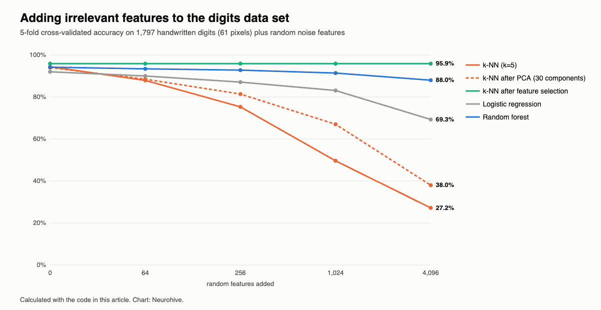
What the experiment shows:
- Distances stop discriminating. The ratio of farthest to nearest distance fell from 135.6 in 2 dimensions to 1.11 in 1,000 and 1.04 in 10,000, and the spread of distances relative to their mean fell from 0.42 to 0.006. In 10,000 dimensions, all 1,000 points are almost exactly as far from the query.
- k-NN collapses under irrelevant features. Accuracy fell from 94.4% to 87.9% with 64 random features, 75.3% with 256, 49.6% with 1,024 and 27.2% with 4,096. The information in the 61 real pixels is still there, but every distance is now dominated by noise.
- PCA is not a cure. Reducing to 30 principal components helped only a little (38.0% at 4,096 noise features), because PCA keeps the directions of largest variance, and with thousands of noise columns those are mostly noise. Unsupervised dimensionality reduction cannot know which variation matters for the label.
- Selecting the right features removes the curse. A simple supervised filter kept the real pixels and gave 95.9% at every noise level, even slightly better than k-NN on the original pixels, because it also dropped a few weak ones.
- Models that choose features suffer less. The random forest, which picks the best feature at each split, still reached 88.0% with 4,096 noise features; logistic regression, which must estimate a weight for every feature from about 1,440 training images, fell to 69.3%, a textbook case of the Hughes phenomenon.
Why deep learning still works
If high-dimensional space is so hostile, how can a network learn from images with millions of pixels, using a few million examples? Several reasons work together:
- The manifold hypothesis. Real data does not fill its space. Random pixel values look like static; natural images, sounds and sentences occupy a tiny, structured region, often described as a low-dimensional manifold inside the high-dimensional space. The effective number of degrees of freedom, such as pose, lighting and shape for a face, is far smaller than the number of pixels.
- Built-in structure. Architectures encode assumptions about the data: convolutional networks assume that nearby pixels are related and that a pattern means the same thing anywhere in the image, which cuts the effective dimensionality dramatically. Embeddings such as word2vec compress huge vocabularies into a few hundred dimensions.
- Gradients instead of search. Gradient descent does not explore the weight space; it follows the slope, so its cost grows linearly with the number of weights.
- The blessing of dimensionality. Some properties of high dimensions help. In very high-dimensional loss landscapes, most points where the gradient is zero are saddle points rather than bad local minima, as Dauphin and colleagues argued in 2014, so gradient descent rarely gets stuck. The concentration of measure behind distance concentration also makes random projections reliable: by the Johnson–Lindenstrauss lemma, n points can be projected into about log(n) / ε² dimensions while keeping all pairwise distances within a factor of 1 ± ε.
The curse does not disappear in deep learning; it moves. Large models need enormous amounts of data, and they work best on data with strong structure, such as images, text and sound. On small tabular data sets with many noisy features, simpler models with good feature selection, such as gradient boosting, often beat neural networks.
The curse of dimensionality in embeddings and vector search
Today the question matters most for embeddings. Retrieval-augmented generation (RAG), semantic search and recommendations turn texts, images and products into vectors and look for the nearest ones. Typical embedding models produce 384 to 4,096 dimensions: OpenAI’s text-embedding-3-large and Google’s Gemini Embedding 2, released in March 2026, both return 3,072 by default. By the distance-concentration argument above, nearest-neighbour search in 3,072 dimensions should be meaningless. In practice it works, for three reasons.
Real data is not uniform noise. The concentration results assume that coordinates are independent and random; real data is correlated and structured. We checked this on the digits: for real images, the farthest image is a median of 4.0 times farther than the nearest, while for uniform noise with the same 61 dimensions and value ranges the ratio is only 1.7. And 21 principal components out of 61 already explain 90% of the variance, so the intrinsic dimension of the data is far lower than the number of pixels.
import numpy as np
from sklearn.datasets import load_digits
from sklearn.decomposition import PCA

rng = np.random.default_rng(0)
X, _ = load_digits(return_X_y=True)
X = X[:, X.std(0) > 0]                                  # 1,797 images, 61 pixels


def contrast(data):
    """Median over 200 queries of farthest / nearest distance to the other points."""
    ratios = []
    for i in rng.choice(len(data), 200, replace=False):
        dist = np.linalg.norm(np.delete(data, i, axis=0) - data[i], axis=1)
        ratios.append(dist.max() / dist.min())
    return np.median(ratios)


uniform = rng.uniform(X.min(0), X.max(0), size=X.shape)   # same ranges, no structure
print(f"farthest/nearest, real digits:   {contrast(X):.2f}")
print(f"farthest/nearest, uniform noise: {contrast(uniform):.2f}")
cum = np.cumsum(PCA().fit(X).explained_variance_ratio_)
for share in [0.80, 0.90, 0.95]:
    print(f"components for {share:.0%} of the variance: {np.searchsorted(cum, share) + 1} of {X.shape[1]}")
farthest/nearest, real digits: 4.02
farthest/nearest, uniform noise: 1.70
components for 80% of the variance: 13 of 61
components for 90% of the variance: 21 of 61
components for 95% of the variance: 29 of 61Good queries are stable. In “Breaking the Curse of Dimensionality: On the Stability of Modern Vector Retrieval” (December 2025), Lakshman, Munyampirwa, Shun and Coleman explain why vector retrieval works in high dimensions: what matters is stability, meaning that a small change to the query does not change its nearest neighbours. When the relevant documents are clearly closer than the rest, as a well-trained embedding model makes them, the results stay meaningful. The authors also show that comparing documents token by token with the Chamfer distance, as multi-vector models such as ColBERT do, keeps this stability, while averaging token vectors into one can destroy it.
Indexes are built for high dimensions. Classic space-partitioning trees such as k-d trees, which are fast in a few dimensions, degrade almost to brute-force search beyond about 20 dimensions, another face of the curse. Vector databases therefore use approximate nearest-neighbour (ANN) indexes: proximity graphs such as HNSW, inverted-file indexes that search only a few clusters, and product quantization, which compresses each vector to a few dozen bytes. They give up a small share of exact neighbours in exchange for speed-ups of orders of magnitude.
Embedding models also fight the curse directly. Matryoshka representation learning (Kusupati et al., 2022), used by text-embedding-3 and Gemini Embedding 2, trains the model so that the first 256, 768 or 1,536 coordinates already form a good embedding: you can truncate vectors to cut storage and search time several times over, with a small loss in quality. Google recommends 3,072, 1,536 or 768 dimensions for Gemini Embedding 2. Use cosine similarity or the dot product on normalized embeddings, the metrics these models are trained for.
How to deal with the curse of dimensionality
- Feature selection. Remove features that carry no information: use domain knowledge, filters such as mutual information or ANOVA F-scores, L1 regularization, or the feature importances of tree models. Fit any selection on the training data only, inside cross-validation, or it will leak information from the test folds.
- Dimensionality reduction. PCA for linear compression of correlated features; autoencoders and learned embeddings for nonlinear structure; random projections for very large, sparse data. Use t-SNE and UMAP to visualize data in 2 or 3 dimensions, but not as input features, because they distort global distances.
- Regularization. L1, L2 and elastic net penalties, dropout and early stopping keep a model with many features from fitting noise.
- More data. When possible, it is the most direct remedy, especially for flexible models.
- Models suited to many features. Tree ensembles and regularized linear models handle irrelevant features better than k-NN; for images, text and sound, architectures with built-in structure.
- Better distances. Scale features, use cosine similarity for embeddings, and learn a metric when distances matter, as in modern vector search.
- Random search for hyperparameters instead of grid search, or Bayesian optimization when trials are expensive.
Most of these tools are part of everyday supervised and unsupervised learning: PCA and clustering on one side, regularized models and feature selection on the other.
FAQ
What is the curse of dimensionality in simple terms?
The more features your data has, the more data you need to cover all their combinations, and the number grows exponentially. With a fixed amount of data, adding dimensions makes the data sparse, makes all points look equally far apart and makes models overfit.
How many dimensions is too many?
There is no fixed number; it depends on the number of examples and on how much of the data’s structure is real. As a rough guide, problems start when the number of features is comparable to the number of samples, or when many features are irrelevant. Distance-based methods already degrade with tens of noisy dimensions, while a regularized model can handle thousands of features if only a few matter.
Does the curse of dimensionality affect k-nearest neighbours?
Yes, more than most algorithms, because k-NN depends entirely on distances. In our experiment, adding 1,024 random features halved its accuracy on the digits data set, from 94.4% to 49.6%, while feature selection restored it completely.
How does PCA help with the curse of dimensionality?
PCA replaces many correlated features with a few components that keep most of the variance, which reduces noise and the number of dimensions. It works when the important information lies in the directions of largest variance; it fails when large, irrelevant noise dominates the variance, as our experiment showed, because PCA does not know the target.
Is the curse of dimensionality the same as overfitting?
No, but they are related. Overfitting is one consequence: with many dimensions and few examples, a model can fit noise. The curse of dimensionality is broader and also covers data sparsity, distance concentration and the exponential cost of search and density estimation.
Do embeddings with thousands of dimensions suffer from the curse of dimensionality?
Less than random data of the same size would, because embeddings are trained so that related items are clearly closer than unrelated ones, and their intrinsic dimension is much lower than their length. Still, exact search over millions of 3,072-dimensional vectors is slow and memory-hungry, which is why vector databases use approximate indexes such as HNSW and why many models allow truncating embeddings to 768 or 1,024 dimensions.
What is the blessing of dimensionality?
The useful side of high dimensions: concentration of measure makes random projections and some statistical estimates reliable, data that is not linearly separable in a few dimensions can become separable in many (the idea behind kernel methods), and high-dimensional loss landscapes have few bad local minima for gradient descent.