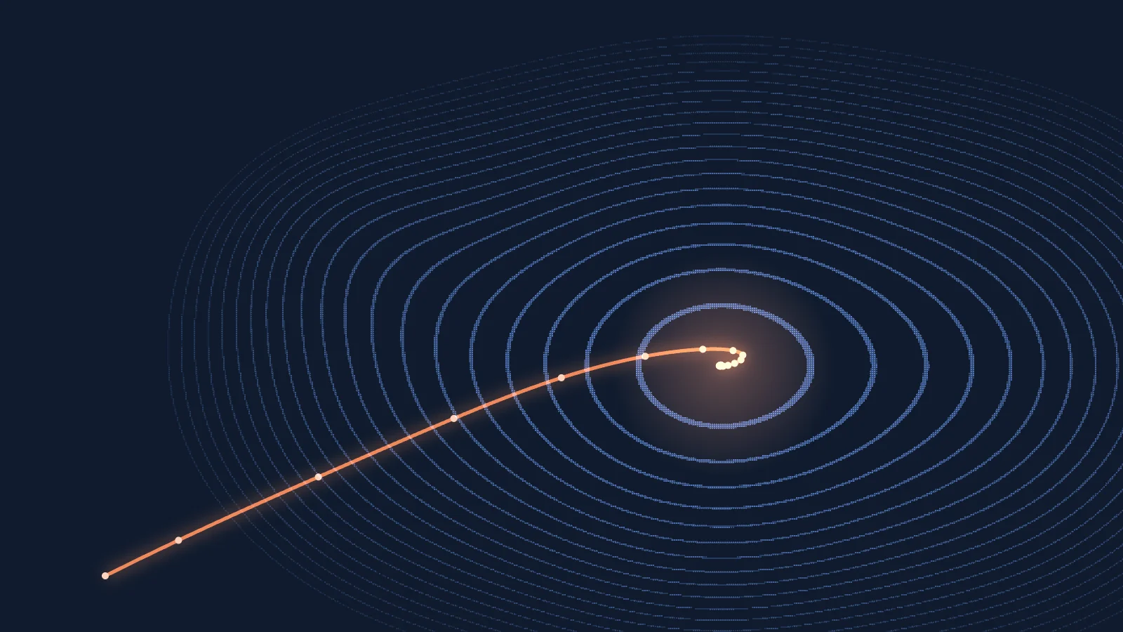
Gradient descent is the algorithm that trains almost every machine learning model: it repeatedly nudges the model’s parameters in the direction that lowers the loss, using the update rule θ ← θ − η · ∇L(θ), where ∇L(θ) is the gradient of the loss and η is the learning rate. Stochastic and mini-batch gradient descent apply the same rule to small random subsets of the data, and optimizers such as momentum, Adam and AdamW are refinements of it.
This guide explains how gradient descent works step by step, how to choose the learning rate, how batch, stochastic and mini-batch variants differ, what momentum, RMSProp, Adam and AdamW add, and how to implement it from scratch in NumPy and with PyTorch optimizers.
Key takeaways
- Idea: compute the slope of the loss with respect to every parameter, then take a small step downhill. Repeat.
- Learning rate is the most important setting: too small and training crawls, too large and the loss oscillates or explodes.
- Mini-batch gradient descent is what everyone uses in practice; “SGD” in deep learning libraries almost always means mini-batch.
- Adam and AdamW adapt the step size for each parameter and are the default optimizers for Transformers and most deep learning models.
- Backpropagation computes the gradients; gradient descent uses them. They are two halves of the same training loop.
What Is Gradient Descent?
Training a model means finding parameters — weights and biases — that make its predictions as accurate as possible. Accuracy is measured by a loss function (also called a cost function), such as mean squared error for regression or cross-entropy for classification. Lower loss means better predictions, so training is an optimization problem: find the parameters that minimize the loss.
For a model with millions or billions of parameters there is no formula that gives the answer directly. Gradient descent solves the problem iteratively. Imagine standing on a hillside in thick fog, trying to reach the valley floor. You cannot see the valley, but you can feel which way the ground slopes under your feet. Take a step in the steepest downhill direction, feel the slope again, take another step. The gradient is that slope: a vector of partial derivatives that points in the direction where the loss increases fastest. Gradient descent moves the opposite way.
The Update Rule, Step by Step
Every iteration applies the same rule to every parameter:
θnew = θold − η · ∂L/∂θ
Here θ is a parameter, ∂L/∂θ is the partial derivative of the loss with respect to it, and η (eta) is the learning rate, which controls the size of the step. The algorithm is:
- Initialize the parameters, usually with small random values.
- Compute the loss on the training data.
- Compute the gradient of the loss with respect to every parameter.
- Update every parameter with the rule above.
- Repeat steps 2–4 until the loss stops improving or a fixed number of iterations is reached.
A one-dimensional example makes this concrete. Take the loss L(w) = (w − 3)², whose minimum is at w = 3. Its derivative is 2(w − 3). Start at w = 0 with a learning rate of 0.1:
| Step | w | Loss (w − 3)² | Gradient 2(w − 3) | Update −0.1 × gradient |
|---|---|---|---|---|
| 0 | 0.000 | 9.000 | −6.000 | +0.600 |
| 1 | 0.600 | 5.760 | −4.800 | +0.480 |
| 2 | 1.080 | 3.686 | −3.840 | +0.384 |
| 3 | 1.464 | 2.359 | −3.072 | +0.307 |
| 4 | 1.771 | 1.510 | −2.458 | +0.246 |
| 5 | 2.017 | 0.966 | −1.966 | +0.197 |
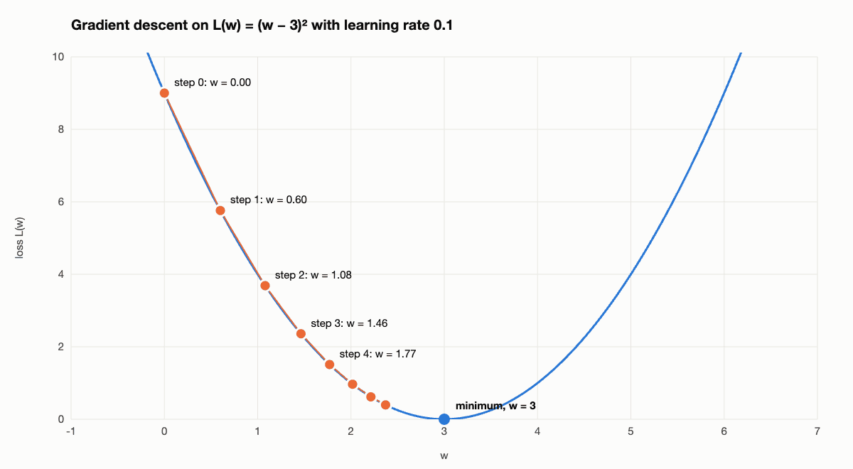
Notice that nobody told the algorithm to slow down. The steps get shorter on their own because the gradient gets smaller near the bottom. After 20 steps w is 2.965, within 1.2% of the true minimum.
Choosing the Learning Rate
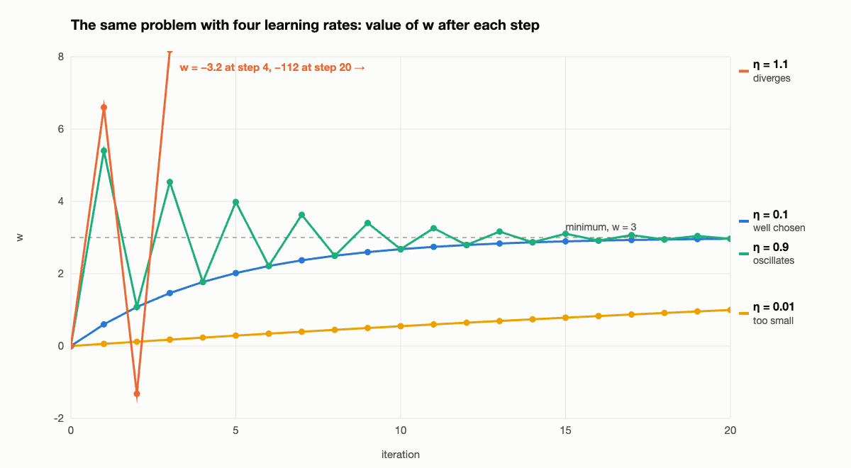
For the same loss, the update can be rewritten as (w − 3) ← (1 − 2η)(w − 3): each step multiplies the distance to the minimum by 1 − 2η. That single factor shows all the ways the learning rate can go wrong:
- Too small (η = 0.01): the distance shrinks by only 2% per step. After 20 steps
wis still 0.997, a third of the way there. - Well chosen (η = 0.1): the distance shrinks by 20% per step and the loss falls smoothly.
- Large (η = 0.9): the factor is −0.8, so
wjumps back and forth across the minimum. It still converges, but by oscillating. - Too large (η = 1.1): the factor is −1.2, so every step overshoots by more than the last. After 20 steps
wis −112 and the loss is exploding.
Real neural networks behave the same way, only in millions of dimensions at once. Common starting points are 0.1 or 0.01 for SGD with momentum and 1e-3 to 3e-4 for Adam; large language models are trained with Adam-family optimizers at small peak learning rates that shrink as the model grows — GPT-3 used 6e-4 for its smallest version and 6e-5 for the 175-billion-parameter model. If the loss becomes NaN or shoots up, the learning rate is the first thing to lower.
Gradient Descent for Linear Regression
Linear regression predicts ŷ = w·x + b and is usually trained with the mean squared error over n examples:
L(w, b) = (1/n) · Σ (w·xᵢ + b − yᵢ)²
Differentiating gives the two gradients gradient descent needs:
∂L/∂w = (2/n) · Σ (w·xᵢ + b − yᵢ) · xᵢ ∂L/∂b = (2/n) · Σ (w·xᵢ + b − yᵢ)
Both are just the average prediction error, weighted by the input for w. Linear regression also has an exact closed-form solution, so it is a convenient test: gradient descent should arrive at the same answer, as the code below shows. For models without a closed form, such as neural networks, gradient descent is the only practical option.
Batch vs Stochastic vs Mini-Batch Gradient Descent
The three classic variants differ only in how much data is used to estimate the gradient for each update.
| Variant | Data per update | Updates per epoch | Gradient | Where it is used |
|---|---|---|---|---|
| Batch (full-batch) | Whole dataset | 1 | Exact, smooth path | Small datasets, convex problems |
| Stochastic (SGD) | 1 example | n | Very noisy | Online learning, historical use |
| Mini-batch | Typically 32–4,096 examples | n / batch size | Noisy but usable | Practically all deep learning |
- Batch gradient descent computes the true gradient over all training examples. Each step is accurate, but a single step on a dataset of millions of images is extremely slow and may not fit in memory.
- Stochastic gradient descent updates after every single example. Updates are cheap and frequent, but the path is very noisy. The noise has a benefit — it can shake the parameters out of shallow local minima and saddle points — but it also prevents settling exactly at the minimum unless the learning rate is gradually reduced.
- Mini-batch gradient descent is the compromise. A batch of tens to thousands of examples gives a reasonable gradient estimate and makes full use of GPU parallelism. When libraries and papers say “SGD”, they almost always mean this. Large language models go further: their batches are counted in millions of tokens.
An epoch is one full pass over the training data. With 50,000 examples and a batch size of 100, one epoch contains 500 updates.
Momentum, RMSProp, Adam and AdamW
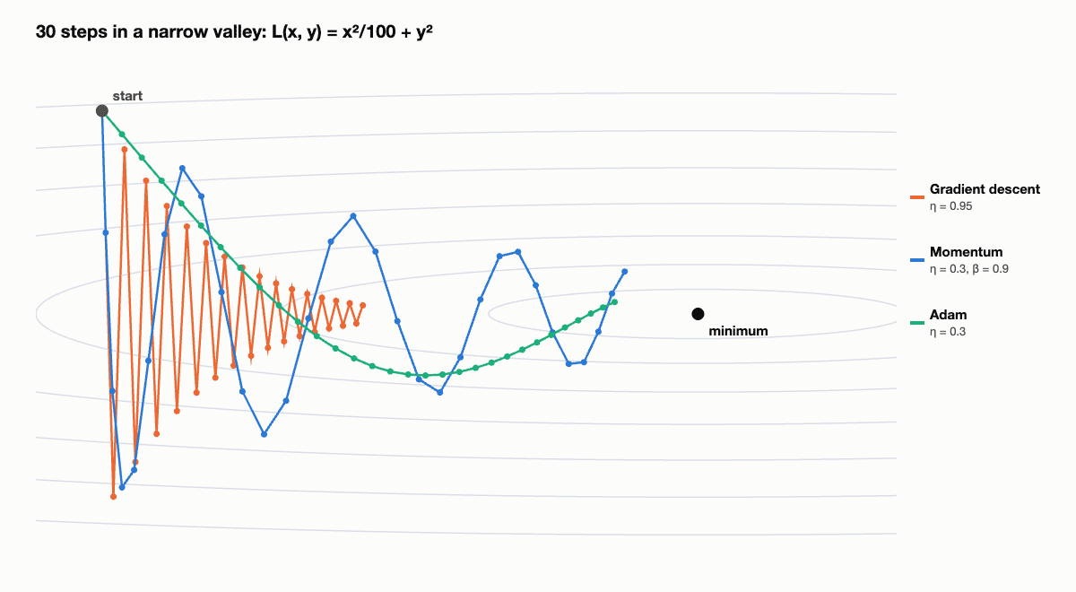
Plain gradient descent struggles when the loss surface is a long, narrow valley: the gradient points mostly across the valley rather than along it, so the parameters zigzag between the walls and make slow progress toward the minimum. Modern optimizers fix this in two ways.
Momentum
Momentum keeps a running average of past gradients, a velocity v ← βv + ∇L, and steps along it: θ ← θ − ηv, with β usually 0.9. Like a ball rolling downhill, it accelerates in directions where the gradient is consistent and dampens the back-and-forth components. SGD with momentum 0.9 trained classic networks such as AlexNet and ResNet, and is still competitive for convolutional networks. Nesterov momentum is a variant that evaluates the gradient slightly ahead of the current position.
RMSProp
RMSProp keeps a running average of the squared gradients for each parameter and divides the step by its square root. Parameters with consistently large gradients get smaller steps, parameters with small gradients get larger ones, so every direction moves at a comparable pace.
Adam
Adam (Kingma and Ba, 2014) combines the two ideas. It tracks a moving average of the gradient (m, the first moment) and of its square (v, the second moment), corrects both for their bias toward zero in the first steps, and updates each parameter with θ ← θ − η · m̂ / (√v̂ + ε). The defaults β₁ = 0.9, β₂ = 0.999 and ε = 1e-8 work for a wide range of problems, which is a large part of its popularity.
AdamW
AdamW (Loshchilov and Hutter) fixes how Adam handles weight decay. In the original Adam, L2 regularization is added to the gradient and then gets rescaled by the adaptive step, which weakens it unevenly. AdamW applies weight decay directly to the weights, separately from the gradient step. It is the standard optimizer for training Transformers, including BERT, GPT-style language models and vision Transformers.
| Optimizer | What it adds | Typical learning rate | Good for |
|---|---|---|---|
| SGD | Nothing: the plain update rule | 0.01–0.1 | Teaching, simple convex problems |
| SGD + momentum | Velocity that smooths the path | 0.01–0.1 | CNNs, when tuned carefully |
| RMSProp | Per-parameter step size | 1e-3 | RNNs, reinforcement learning |
| Adam | Momentum + per-parameter step size | 1e-3 to 3e-4 | Default for most deep learning |
| AdamW | Adam with decoupled weight decay | 1e-4 to 1e-3 | Transformers and LLMs |
Learning Rate Schedules and Warmup
A fixed learning rate is rarely optimal. Early in training, large steps make fast progress; later, smaller steps let the parameters settle into a good minimum instead of bouncing around it. A learning rate schedule changes η over time:
- Step decay divides the learning rate by a constant, often 10, at fixed epochs or when the validation loss stops improving. ResNet was trained this way.
- Cosine decay lowers the learning rate smoothly along a half cosine curve from its peak to near zero. It is the most common schedule for training large models.
- Warmup starts from a very small learning rate and increases it linearly over the first few hundred or thousand steps. Adam’s statistics are unreliable at the very beginning of training, and warmup prevents early instability. Transformers are almost always trained with warmup followed by cosine or linear decay.
Local Minima, Saddle Points and Convexity
If the loss is a convex function — shaped like a single bowl, as for linear regression and logistic regression — every local minimum is the global minimum, and gradient descent with a suitable learning rate is guaranteed to find it.
Neural network losses are not convex. They can have many local minima, points that are lower than everything around them but not the lowest overall. In high-dimensional networks, however, research has found that the bigger obstacle is usually saddle points: places where the gradient is zero but the surface curves up in some directions and down in others. Gradient descent slows down near them because the gradient is tiny. Noise from mini-batches and momentum both help escape, and in practice the minima that large networks reach tend to generalize similarly well.
Gradient ascent is the same algorithm with the sign flipped, θ ← θ + η∇f, used when you want to maximize a function instead — for example, a reward in reinforcement learning or a likelihood in statistics.
Gradient Descent and Backpropagation
The two terms are often confused. Backpropagation is the algorithm that computes the gradient of the loss with respect to every weight in a neural network, by applying the chain rule layer by layer from the output back to the input. Gradient descent is the algorithm that uses those gradients to update the weights. In a PyTorch training loop, loss.backward() is backpropagation and optimizer.step() is the gradient descent update.
Gradient Descent in Python
From scratch with NumPy
The function below fits a line to noisy data generated from y = 3x + 5. Setting batch_size switches between batch, mini-batch and stochastic gradient descent:
import numpy as np

rng = np.random.default_rng(0)
X = rng.uniform(0, 10, size=200)
y = 3 * X + 5 + rng.normal(0, 2, size=200)   # true slope 3, intercept 5

def gradient_descent(X, y, lr=0.01, epochs=1000, batch_size=None):
    w, b = 0.0, 0.0
    n = len(X)
    batch_size = batch_size or n                # None = full batch
    for epoch in range(epochs):
        idx = rng.permutation(n)
        for start in range(0, n, batch_size):
            j = idx[start:start + batch_size]
            error = (w * X[j] + b) - y[j]
            dw = 2 * np.mean(error * X[j])      # dL/dw for mean squared error
            db = 2 * np.mean(error)             # dL/db
            w -= lr * dw
            b -= lr * db
    mse = np.mean((w * X + b - y) ** 2)
    return w, b, mse

print("batch:      w=%.3f b=%.3f mse=%.3f" % gradient_descent(X, y, lr=0.01, epochs=2000))
print("mini-batch: w=%.3f b=%.3f mse=%.3f" % gradient_descent(X, y, lr=0.01, epochs=200, batch_size=32))
print("SGD:        w=%.3f b=%.3f mse=%.3f" % gradient_descent(X, y, lr=0.001, epochs=50, batch_size=1))
print("lstsq:      w=%.3f b=%.3f" % tuple(np.polyfit(X, y, 1)))
Output:
batch:      w=2.949 b=5.094 mse=4.169
mini-batch: w=3.019 b=5.113 mse=4.369
SGD:        w=2.897 b=5.044 mse=4.305
lstsq:      w=2.949 b=5.094
Full-batch gradient descent lands exactly on the least-squares solution. Mini-batch and stochastic versions get close but keep jittering around it because each update sees only part of the data — which is why their learning rate is usually decayed toward the end of training.
With PyTorch optimizers
In PyTorch you never write the update by hand. Every optimizer in torch.optim implements a variant of the same rule, and the training loop is identical for all of them:
import torch
import torch.nn as nn

torch.manual_seed(0)
X = torch.rand(200, 1) * 10
y = 3 * X + 5 + torch.randn(200, 1) * 2

def train(make_optimizer, steps=500):
    model = nn.Linear(1, 1)
    optimizer = make_optimizer(model.parameters())
    loss_fn = nn.MSELoss()
    for step in range(steps):
        optimizer.zero_grad()            # clear old gradients
        loss = loss_fn(model(X), y)      # forward pass
        loss.backward()                  # backpropagation computes the gradients
        optimizer.step()                 # one gradient descent update
    return model.weight.item(), model.bias.item(), loss.item()

optimizers = {
    "SGD":          lambda p: torch.optim.SGD(p, lr=0.01),
    "SGD+momentum": lambda p: torch.optim.SGD(p, lr=0.01, momentum=0.9),
    "Adam":         lambda p: torch.optim.Adam(p, lr=0.1),
    "AdamW":        lambda p: torch.optim.AdamW(p, lr=0.1, weight_decay=0.01),
}
for name, make in optimizers.items():
    w, b, loss = train(make)
    print(f"{name:>13}: w={w:.3f} b={b:.3f} loss={loss:.3f}")
Output (PyTorch 2.14):
          SGD: w=3.084 b=4.353 loss=4.484
 SGD+momentum: w=3.038 b=4.651 loss=4.460
         Adam: w=3.055 b=4.543 loss=4.463
        AdamW: w=3.054 b=4.454 loss=4.477
The exact least-squares answer for this data is w = 3.038, b = 4.651. After 500 steps SGD with momentum has reached it, while plain SGD is still crawling toward the right intercept: the input is not normalized, so the gradient for the bias is much smaller than for the weight. Standardizing the features would let plain SGD converge just as fast.
Practical Tips
- Normalize the inputs. Features on very different scales create narrow valleys in the loss surface and slow gradient descent down, as the PyTorch example shows.
- Start with AdamW at a learning rate around 3e-4 for a new deep learning model, then tune. Try SGD with momentum if you are training a CNN and have time to tune the schedule.
- If the loss is NaN or explodes, lower the learning rate, add warmup, or clip gradients with
torch.nn.utils.clip_grad_norm_. - If the loss barely moves, the learning rate may be too small, the gradients may be vanishing, or there may be a bug: check that you call
optimizer.zero_grad()every step and that the model is in training mode. - Overfit a tiny batch first. A correct model and optimizer should drive the loss on 10–20 examples close to zero. If they cannot, something is broken before any tuning matters.
FAQ
What is gradient descent in simple terms?
It is a way to find the minimum of a function by repeatedly taking small steps downhill. In machine learning the function is the loss, and the steps adjust the model’s weights so its predictions become more accurate.
What is the difference between gradient descent and stochastic gradient descent?
Gradient descent computes the gradient on the whole training set before each update. Stochastic gradient descent estimates it from a single example, or in modern usage from a small mini-batch, which makes each update far cheaper at the cost of noise.
Is Adam better than SGD?
Adam usually converges faster and needs less tuning, which is why it is the default for Transformers. Well-tuned SGD with momentum can match or beat it on some vision tasks and sometimes generalizes slightly better. AdamW is a safe first choice.
What learning rate should I use?
There is no universal value. Common starting points are 1e-3 or 3e-4 for Adam and AdamW, and 0.1 or 0.01 for SGD with momentum. Use a learning rate finder or a short sweep, and combine the chosen value with warmup and a decay schedule.
Does gradient descent always find the global minimum?
Only for convex problems such as linear and logistic regression. For neural networks it finds a good local minimum or a flat region, which in practice is usually good enough.
See also: how classic networks were trained with SGD and momentum in our breakdowns of AlexNet, VGG16 and ResNet.